A VARIANT ON THE GRAPH PARAMETERS OF COLIN DE
VERDI`ERE: IMPLICATIONS TO THE MINIMUM RANK OF
GRAPHS∗
FRANCESCO BARIOLI†, SHAUN FALLAT‡,AND LESLIE HOGBEN§
Abstract. For a given undirected graphG, the minimum rankofGis defined to be the smallest possible rankover all real symmetric matricesAwhose (i, j)th entry is nonzero wheneveri=jand
{i, j}is an edge inG. Building upon recent workinvolving maximal coranks (or nullities) of certain symmetric matrices associated with a graph, a new parameterξis introduced that is based on the corankof a different but related class of symmetric matrices. For this new parameter some properties analogous to the ones possessed by the existing parameters are verified. In addition, an attempt is made to apply these properties associated withξto learn more about the minimum rankof graphs – the original motivation.
Key words. Graphs, Minimum rank, Graph minor, Corank, Strong Arnold property, Symmetric matrices.
AMS subject classifications. 15A18, 05C50.
1. Introduction. Recent work and subsequent results have fueled interest in important areas such as spectral graph theory and certain types of inverse eigenvalue problems. Of particular interest here is to bring together some of the pioneering work of Y. Colin de Verdi`ere (specifically his parameter related to planarity of graphs) and the minimum rank of graphs.
All matrices discussed in this paper are real and symmetric. IfA∈Mn is a fixed symmetric matrix, thegraph ofAdenoted byG(A), has{1, ..., n}as vertices, and as edges the unordered pairs{i, j} such thataij = 0 withi=j. GraphsGof the form
G=G(A) do not have loops or multiple edges, and the diagonal of A is ignored in the determination ofG(A). Similarly, for a given graphG, we let
S(G) ={A∈Mn|A=AT, G(A) =G}.
Finally, for any symmetric matrixA∈Mn, we letSA=S(G(A)).
Suppose thatGis a graph on nvertices. Then theminimum rank ofGis given by
mr(G) = min
A∈S(G)rankA.
∗Received by the editors 27 May 2005. Accepted for publication 29 November 2005. Handling
Editor: Richard A. Brualdi.
†Department of Mathematics, University of Tennessee at Chattanooga, Chattanooga TN, 37403
‡Department of Mathematics and Statistics, University of Regina, Regina, SK, Canada
([email protected]). Research supported in part by an NSERC research grant.
§Department of Mathematics, Iowa State University, Ames, IA 50011, USA
It is not difficult to verify that mr(G) = n−M(G), whereM(G) is the maximum
multiplicity ofG, and is defined to be
M(G) = max
A∈S(G){multA(λ) :λ∈σ(A)}.
Furthermore it is easy to see that for any graph, max{corankA|A∈ S(G)}=M(G), where corankA is defined to be the nullity of A. Hereσ(A) denotes the spectrum of A and multA(λ) is the multiplicity of λ ∈ σ(A). Also, if W ⊂ {1,2, . . . , n} and A∈Mn, thenA[W] means the principal submatrix ofAwhose rows and columns are indexed byW, andA(W) is the complementary principal submatrix obtained fromA
by deleting the rows and columns indexed byW. In the special case when W ={v}
a singleton, we let A(v) = A(W). For a fixed m×nmatrix A, R(A) and Null(A) denote the range and the null space ofA, respectively.
An interesting and still rather unresolved problem is to characterize mr(G) for a given graphG. Naturally, there have been a myriad of preliminary results, which take on many different forms. For example, if Pn,Cn, Kn, En, denote the path on
nvertices, the cycle onn vertices, the complete graph onnvertices, and the empty (edgeless) graph onnvertices, respectively, then
mr(Pn) =n−1, mr(Cn) =n−2, mr(Kn) = 1, mr(En) = 0.
Further it is well known that for any connected graphGonnvertices that mr(G) = 1 if and only ifGisKn. Fiedler [8] established that mr(G) =n−1 if and only if Gis
Pn. Barrett, van der Holst, and Loewy [4] have characterized all of the graphs onn
vertices that satisfy mr(G) = 2.
Other important work pertaining to the class of trees [11], states that mr(T) =
n−P(T), where P(T) is the path cover number, namely, the minimum number of vertex disjoint paths occurring as induced subgraphs ofT, that cover all the vertices ofT. More recently, some modest extensions along these lines have been produced for graphs beyond the class of trees. Namely, for vertex sums and edge sums of so-called non-deficient graphs (which include trees), and for the case of unicyclicgraphs, i.e., graphs that contain a unique cycle [2, 3].
On a related topic there has been some extremely interesting and exciting work on spectral graph theory that is connected to certain aspects of planarity. For a given graph, a matrix L = [lij] ∈ S(G) is called a generalized Laplacian matrix of Gif for i =j, lij <0 whenever i, j are adjacent in Gand lij = 0 otherwise. Colin de Verdi`ere introduced the parameter µ(G) associated with the nullity of certain generalized Laplacian matrices inS(G) (see [5, 9, 10] for more specific details). The paper [10] provides a clear exposition and survey of these results, and we will follow much of the notation and treatment given in that paper. The actual definition of
µ(G) will be presented below.
We now turn our attention to the so-calledStrong Arnold Property, which will be shortened to SAP throughout. We will see that it plays a crucial role in monotonicity, such as the subgraph monotonicity ofµ.
We say two matrices are orthogonal if, when viewed as n2-tuples in Rn2
if and only if trace(ATB) = 0. The matrixB isorthogonal to the family of matrices F ifB is orthogonal to every matrix C∈ F. A family we will consider frequently is
F =S(G) where G is a graph; X orthogonal to S(G) requires that every diagonal entry ofX is 0 and for every edge ofG, the corresponding off-diagonal entry ofX is 0. Recall that, ifA= [aij] andB= [bij] are matrices inMn, the matrixA◦Bdefined by [A◦B]ij =aijbij is called theHadamard productofAandB.
Definition 1.1. Let A, X be symmetricn×n matrices. We say thatX fully
annihilatesA if
1. AX= 0; 2. A◦X = 0; 3. In◦X= 0.
In other words,X fully annihilatesAifX is orthogonal toSA andAX= 0. Definition 1.2. The matrix A has the Strong Arnold Property (SAP) if the zero matrix is the only symmetric matrix that fully annihilatesA.
We begin with a basic, yet useful, observation concerning low corank. Lemma 1.3. If corankA1, then Ahas SAP.
Proof. If corankA = 0, then A is nonsingular, and the only matrix X that
fully annihilatesA is the zero matrix. Suppose now corankA = 1, and let X fully annihilateA. Therefore, the diagonal of X is 0. SinceX is symmetric, this implies
X is not a rank 1 matrix. Thus ifX = 0, then rankX 2, andAX= 0 would imply corankA2. ThusX = 0 andAhas SAP.
We are now in a position to formally define the Colin de Verdi`ere parameter,
µ(G). For a given graphG, µ(G) is defined to be the maximum multiplicity of 0 as an eigenvalue ofL, where Lsatisfies:
1. L∈ S(G), and is a generalized Laplacian matrix;
2. Lhas exactly one negative eigenvalue (with multiplicity one); 3. Lhas SAP.
In other words µ(G) is the maximum corank among the matrices satisfying (1)-(3) above. Further observe that µ(G)M(G) =n−mr(G). Hence there is an obvious relationship betweenµ(G) and mr(G).
Colin de Verdi`ere and others ([5, 9, 10]) have shown that
• µ(G)1 if and only ifGis a disjoint union of paths,
• µ(G)2 if and only ifGis outerplanar,
• µ(G)3 if and only ifGis planar,
• µ(G)4 if and only ifGis linklessly embeddable.
A related parameter, also introduced by Colin de Verdi`ere [6] is denoted byν(G), and is defined to be the maximum corank among matricesAthat satisfy:
1. A∈ S(G);
2. Ais positive semidefinite; 3. Ahas SAP.
Properties analogous to µ(G) have been established for ν(G). For example,
ν(G) 2 if the dual of G is outerplanar, see [6]. Furthermore, ν(G), like µ(G) is graph minor monotone – we will come back to this issue later.
introduce the following new parameter, which we denote byξ(G).
Definition 1.4. For a graph G, ξ(G) is the maximum corank among matrices
A∈ S(G)having SAP.
For a graph parameter ζ defined to be the maximum corank over a family of matrices associated with graph G, we say A isζ-optimal for GifA is in the family and corankA=ζ(G).
Remark 1.5. Since for any graph G, any µ-optimal orν-optimal matrix for G is inS(G) and has SAP,µ(G)ξ(G) andν(G)ξ(G).
In Example 3.11 we determine a graph G such that µ(G) < ξ(G) and ν(G) < ξ(G). For motivational purposes and completeness, we give several examples and observations on the evaluation ofξ.
Observation 1.6. ξ(G) = 1 exactly whenGis a disjoint union of paths. Indeed, ifξ(G) = 1, we haveµ(G)1, so that Gis a disjoint union of paths. On the other hand, since M(Pn) = 1, and any corank 1 matrix has SAP, ξ(Pn) = 1. Then, the converse will follow easily from Theorem 3.2, in which we show thatξ of a disjoint union is the maximum value ofξon the components.
Observation 1.7. If n > 1, ξ(Kn) = n−1, because J, the all 1’s matrix, is in S(Kn), has corank n−1, and has SAP (any matrix in S(Kn) has SAP since a matrix orthogonal to S(Kn) is necessarily 0). ξ(K1) = 1 because any corank 1 matrix has SAP. Conversely, it is well known that the only connected graph having
M(G) =|G| −1 isKn, so (again using Theorem 3.2)ξ(G) =|G| −1 impliesG=Kn
orG=K2, the complement ofK2, also denoted byE2.
Example 1.8. ξ(Cn) = 2, because M(Cn) = 2 (see for example [2, 3]) so
ξ(Cn)2, butCn is not a disjoint union of paths soξ(Cn)2.
The next example shows that it is possible to have a matrixAthat isξ-optimal for graphG, and another matrixB∈ S(G) with corankA= corankBbutBdoes not have SAP. It also illustrates how computations to establish SAP (or find a matrixX
showing failure to have SAP) can be performed.
s
3
s
1
s
4
s
5
s
2
s
[image:4.595.239.347.560.628.2]6
Fig. 1.1.A graph withB∈ S(G),corankB=ξ(G), butBdoes not have SAP
Let A=
1 2 1 1 0 0
2 8 0 0 −3 1
1 0 0 0 0 0
1 0 0 0 0 0
0 −3 0 0 1 0
0 1 0 0 0 −1
; B=
1 2 1 1 0 0
2 8 0 0 −3 1
1 0 0 0 0 0
1 0 0 0 0 0
0 −3 0 0 0 0
0 1 0 0 0 0
.
ClearlyA, B ∈ S(G), and direct computation shows corankA= corankB = 2. The matrix X=
0 0 0 0 0 0
0 0 0 0 0 0
0 0 0 0 −1
3 −1
0 0 0 0 1
3 1
0 0 −1
3 1
3 0 0
0 0 −1 1 0 0
fully annihilatesB, so thatBdoes not have SAP. To showAdoes have SAP (and thus isξ-optimal forG), computeAX for an arbitrary symmetric matrixX orthogonal to
S(G). An examination of the last two columns of AX showsx15 =x16 =x56 = 0. The second, third and fourth entries of the first row arex23+x24,2x23+x34,2x24+x34, forcingx23 =x24 =x34 = 0. After substituting these values, we see from the third and fourth columns thatx35=x36=x45=x46= 0. In other words,X = 0.
Example 1.10. IfGis regular of degree|G| −2, thenξ(G) =M(G), since any matrixA∈ S(G) has SAP (ifX is orthogonal toS(G), at most one entry in any row is nonzero, which implies easilyX = 0).
Example 1.11. IfT is a tree that is not a path, then ξ(T) = 2. This will be proved in Theorem 3.7.
Example 1.12. LetKp,q denote the complete bipartite graph on sets ofpandq vertices, 1pq. Observe thatξ(K1,1) =ξ(P2) = 1, and thatξ(K1,2) =ξ(P3) = 1. If q 3, thenξ(Kp,q) = p+ 1, as will be proved in Corollary 2.8, while ξ(K2,2) =
ξ(C4) = 2.
The tools we use to exploit SAP come from manifold theory. As in [10], let
M1, . . . , Mkbe open manifolds embedded inRd, and letxbe a point in their intersec-tion. We sayM1, . . . , Mk intersect transversally at xif their normal spaces atxare independent. That is, ifni is orthogonal toMi fori= 1, . . . , kandn1+· · ·+nk= 0, thenni = 0 for alli= 1, . . . , k. A smooth family of manifoldsM(t) in Rd is defined by a smooth functionf:U×(−1,1)→Rd, where U is an open set inRs(sd−1), and for each−1< t <1, the function f(·, t) is a diffeomorphism betweenU and the manifoldM(t).
For a givenn×nmatrixA, letRA be the set of alln×nmatricesB such that rankB= rankA. The next lemma is from [10].
Lemma 1.13. The matrix A has SAP if and only if the manifolds RA and SA
The next lemma is a slightly simplified version Lemma 2.1 of [10].
Lemma 1.14. Let M1(t), . . . , Mk(t) be smooth families of manifolds in Rd and
assume that M1(0), . . . , Mk(0) intersect transversally at x. Then there exists ǫ >
0 such that for any t such that |t| < ǫ, the manifolds M1(t), . . . , Mk(t) intersect
transversally at a pointx(t)so that x(0) =xandx(t)depends continuously on t.
Lemma 1.15. [10, Cor. 2.2] Assume that M1, . . . , Mk are manifolds inRd that
intersect transversally atx, and assume that they have a common tangent vectorv at
xwithv= 1. Then for everyǫ >0there exists a pointx′=xsuch thatM
1, . . . , Mk
intersect transversally at x′, and
(x−x
′) x−x′ −v
< ǫ.
In Section 2 we establish a graph monotonicity property for ξ, which is also possessed by both µand ν. In Section 3, from the results in Section 2, we build up many useful tools and facts aboutξ and use them to learn more aboutξ, and apply these results to mr(G).
2. Minor Monotonicity and Consequences. Following the previous works of Colin de Verdi`ere as described in [10], we prove that the parameter introduced here, ξ, is also graph minor monotone. We begin with a preliminary result, which also follows from the results in Section 3.
Observation 2.1. ξ is monotone for deletion of an isolated vertex, i.e., ifG′ is obtained fromGby deleting an isolated vertex ofG, then ξ(G′)ξ(G).
Proof. LetG′be obtained fromGby deleting an isolated vertexvofG. Choose a
ξ-optimal matrixA′ forG′. It is sufficient to construct a matrixA∈ S(G) such that
corankA= corankA′ andAhas SAP, for thenξ(G)corankA= corankA′=ξ(G′).
Let Abe the matrix obtained from A′ by adding (in position v) a row and column
consisting of 0s exceptAv,v = 1. Then clearlyA∈ S(G), corankA= corankA′, and
a simple computation showsAhas SAP.
Theorem 2.2. ξ is edge deletion monotone, i.e., if G′ is obtained from G by
deleting an edge ofG, thenξ(G′)ξ(G).
Proof. Let G′ be obtained from G by deleting edge {u, w}. Proceeding as in
Observation 2.1, we choose a ξ-optimal matrixA′ forG′ and construct the required
matrix A ∈ S(G). Since A′ has SAP, the two manifolds RA
′ and SA′ intersect
transversally atA′. LetS(t) be the manifold obtained fromSA
′ by replacing (in each
matrix in SA′) the 0s in positions (u, w) and (w, u) by t. LetR(t) =RA′. Then by
Lemma 1.14, for a sufficiently small positive t, R(t) and S(t) intersect transversally atA=A(t). ThusAhas SAP. SinceA∈ R(t) =RA′, we have corankA= corankA′,
and sinceA∈ S(t),A∈ S(G).
Corollary 2.3. ξ is subgraph monotone, i.e., if G′ is a subgraph of G, then ξ(G′)ξ(G).
Recall that for a given edgee={u, v}ofGwe saycontracteinGto mean delete
Theorem 2.4. ξ is contraction monotone, i.e., if G′ is obtained from G by
contracting an edge, thenξ(G′)ξ(G).
Proof. Let |G| = n, suppose{1,2} ∈ E(G), and let G′ be obtained from G by
contracting {1,2} (call this new vertexv and place it first in order of the vertices ofG′). If vertex 1 is adjacent only to vertex 2, then the result follows by subgraph
monotonicity. So we may assume 1 is adjacent to at least one vertex in addition to 2. Renumber if necessary so that vertex 1 is adjacent exactly to the vertices 2,3, . . . , r
(r3). By the edge monotonicity of ξ, without loss of generality, we may assume vertex 2 is not adjacent to any of the vertices 3, . . . , r. Ann×n symmetric matrix will be written in the following block form
B=
b11 b12 bT1 b′T1
b12 b22 bT2 b′T2 b1 b2
b′
1 b′2
B0 ,
whereb1∈Rr−2. In addition, let U be the 0-1 matrix with G(U) =G′ andUii = 1
for eachi. We then have
U =
1 1T u′T2 1
u′
2
U0 ,
where1denotes the vector all of whoser−2 entries are equal to 1, whileu′
2 (U0) is a suitable 0-1 vector (matrix).
We define three manifolds as follows.
• M1 is the set ofn×nsymmetric matricesB such thatb12= 0,b′1= 0 and
B(1)◦U = B(1), that is, G(B(1)) can be obtained from G′ by (possibly)
removing some edges.
• M2is the set of n×nsymmetric matricesB such that corankB=ξ(G′).
• M3is the set of n×nsymmetric matricesB such that rank[b1 b2] = 1. As shown in [10],
• ifB∈ M1, the normal space ofM1atB is the set of symmetric matricesX such that
X =
0 x12 0T x′T1
x12 0 xT2 x′T2
0 x2
x′
1 x′2
X0
, X(1)◦U = 0; (2.1)
• ifB∈ M2, the normal space ofM2atB is the set of symmetric matricesY such that
• if B ∈ M3, and b1 = γb2, the normal space of M3 at B is the set of symmetric matricesZ such that
Z=
0 0 zT
1 0T 0 0 −γzT1 0T z1 −γz1
0 0 0
, z
T
1b2= 0. (2.3)
Define
P =
1 0 0T 0T
0 p22 pT2 p′T2 0 p2
0 p′
2
P0 ,
where P(1) is a ξ-optimal matrix for G′. Note that rankP = 1 + rankP(1); so
corankP =ξ(G′). In addition,P is in each of the Mi’s (note thatp2 = 0, so that P ∈ M3). As shown in [10], the three manifolds intersect transversally atP, and the matrix
T =
0 0 pT
2 0T 0 0 0T 0T p2 0
0 0 0
is a common tangent to all three manifolds at P. Thus, by Lemma 1.15 (or [10, Cor. 2.2]), there is a matrix Q in the intersection of the Mi’s such that the Mi’s intersect transversally at Q, and Q−P is “almost parallel” to T. By a judicious choice ofǫ, we can ensure thatQhas nonzero entries everywhereP orT has nonzero entries. In other words we can write
Q=
q11 0 qT1 0T 0 q22 qT2 q′T2 q1 q2
0 q′2
Q0 ,
where G(Q(1)) = G′. In particular, q2 has no zero components. Moreover, since Q∈ M3, there exists γ= 0 such thatq1 =γq2, so that q1 has no zero components as well.
LetS =In− 1
γE21, andA=SQST. Easy computations show that G(A) =G,
and corankA= corankQ=ξ(G′). So it is enough to show thatAhas SAP. Suppose,
A. ThenA◦W = 0 and In◦W = 0, so that
W =
0 0 0T w′T1
0 0 wT
2 w′T2
0 w2
w1′ w′2
W0 .
In additionAW = 0, that is, SQSTW = 0, and since S is invertible, we can write QSTW S= 0. Defi ne
Y =STW S=
0 0 −1γwT
2 w1′T−γ1w′T2
0 0 wT2 w′T2
−1
γw2 w2
w′
1−1γw′2 w′2
W0
.
Ifw2= 0, define further
Z=
0 0 −1
γwT2 0T
0 0 wT
2 0T
−1γw2 w2
0 0 0
,
and X = Y −Z. By using (2.1), (2.2), and (2.3), we see that X, Y, and Z are normal at Q to M1, M2, andM3, respectively, so that the Mi’s do not intersect transversally atQ, which is a contradiction. On the other hand, if w2= 0,Y would be normal atQto bothM1 andM2, which is again a contradiction.
For a given graphG, we callHaminor of GifHis obtained fromGby a sequence of deletions of edges, deletions of isolated vertices, and contractions of edges. We are now in a position to state the minor monotonicity result ofξwhich bothµandν also satisfy.
Corollary 2.5. ξis minor monotone, i.e., ifG′ is a minor ofG, thenξ(G′) ξ(G).
As noted in [10], this implies that the Robertson-Seymour graph minor theory applies toξ, so that the graphsGthat have the propertyξ(G)kcan be characterized by a finite set of forbidden minors. The Robertson-Seymour graph minor theorem is an extremely powerful tool; consult the last chapter [7] for further discussion.
Using the results thus far, we continue to derive more properties of the parameter
ξ, while at the same time adding to the list of examples in whichξcan be calculated. The first result below is a direct consequence of Corollary 2.3 and Observation 1.7.
Corollary 2.6. If Kp is a subgraph of G thenξ(G)p−1.
Corollary 2.7. Suppose V(G) has disjoint subsetsWi, i = 1, . . . , q such that
for all i = 1, . . . , q the subgraph of G induced by Wi is a path, and for all i = j,
|G| −(|W1|+. . .+|Wq|) + 1. In particular, if G has a set ofq independent vertices
(i.e., eachWi is a singleton), thenξ(G)|G| −q+ 1.
Proof. Label the vertices inWithat are the endpoints of the path induced byWias
uiandvi(if|Wi|= 1 thenui=vi; otherwise they are distinct). Create a new graphG′
by adding the edges{vi, ui+1}fori= 1, . . . , q−1. Since there is no edge inGbetween a vertex in Wi and a vertex in Wj, the subgraphH induced inG′ by q
i=1Wi is a path on|W1|+. . .+|Wq|vertices, so mrH=|W1|+. . .+|Wq| −1. SinceH is induced, mr(H)mr(G′), soM(G′) =|G′| −mr(G′)|G| −(|W
1|+. . .+|Wq|) + 1. By edge monotonicity (Theorem 2.2),ξ(G)ξ(G′)M(G′)|G| −(|W
1|+. . .+|Wq|) + 1. Sinceµ(G), ν(G)ξ(G), any graphGsatisfying the hypotheses of Corollary 2.7 also hasµ(G)|G| −(|W1|+. . .+|Wq|) + 1 andν(G)|G| −(|W1|+. . .+|Wq|) + 1. The next corollary follows from the previous one and the facts thatµ(Kp,q) =p+1 forqp1 andq3 [10], andµ(G)ξ(G) for any graphG.
Corollary 2.8. If qp1 andq3 thenξ(Kp,q) =p+ 1.
The next corollary is an immediate consequence of edge monotonicity. Note that the only distinction between matrices considered when maximizing corank forM and forξis SAP.
Corollary 2.9. If it is possible to add an edge to G, obtaining graph G′,
and have M(G′) < M(G) then ξ(G) < M(G), i.e., any matrix A in S(G) with
rankA= mr(G)does not have SAP.
We have seen that SAP is sufficient for edge monotonicity. In fact, SAP also appears to be necessary for edge monotonicity; we have results for several families of graphsGthat whenξ(G)< M(G), it is possible to add an edge and reduce M. For example, the proof of Corollary 2.7 shows how to add edges between theqindependent vertices ofKp,q to obtain a graphG with M(G)< M(Kp,q), providedq4. Note that it follows from Corollary 2.8 thatξ(Kp,q)< M(Kp,q) is true exactly whenq4. We do not know of any examples withξ(G)< M(G) where it is not possible to add an edge and reduceM (see also Proposition 3.8).
3. Constructions. In this section we examine the behavior ofξ under various constructions, such as disjoint union, vertex sum, joins, etc. In contrast to the previ-ous section, where the results closely paralleled those forµ, and where the methods of proof were often the same as those in [10], here the results for ξsometimes differ from those forµ, and in most cases even when the result is the same, the method of proof is different. We will need numerous technical lemmas.
Lemma 3.1. Let B be the direct sum of matrices Bi, i= 1, . . . , k. Then B has
SAP if and only if at most oneBi is singular, and suchBi has SAP.
Proof. LetB have SAP, and suppose two of theBi, sayB1andB2, are singular.
Then there exist nonzero vectors x1, x2 such that B1x1 = B2x2 = 0. Let ˆx1 = [xT
1 0 0]T and ˆx2= [0 xT2 0]T. ThenX = ˆx1xˆT2 + ˆx2xˆT1 fully annihilatesB, so that
B does not have SAP. Therefore, at most one of theBi, sayB1, is singular. Suppose now that B1 does not have SAP. Then, there exists a nonzero matrix X1 that fully
annihilates B1, so that the matrixX = X01 00
fully annihilates B, that is, B
Conversely, if all Bi are nonsingular, then B is nonsingular, and has SAP by Lemma 1.3. If exactly one of the Bi, say B1, is singular and has SAP, then we
can write B = B1 0 0 B′
, where B′ is nonsingular. LetX = X11 X21T
X21 X22
fully
annihilateB. Then BX = 0 implies B′X
21 = B′X22 = 0, that is, X21 = X22 = 0. Thus we haveB1X11 = 0, and, finally, X11 = 0, since B1 has SAP. In other words,
X is necessarily the zero matrix, so that B has SAP.
The next theorem follows immediately from Lemma 3.1 and the monotonicity of
ξon submatrices. The analogous result is true forµ.
Theorem 3.2. If Gis not connected, and the components of G are the graphs
G1, . . . , Gk, thenξ(G) = maxki=1ξ(Gi). Lemma 3.3. Let
B=
β cT1 cT2 cT3
c1 B1 0 0
c2 0 B2 0
c3 0 0 B3
,
and suppose Null c
T i Bi
= 0for i= 1,2. ThenB does not have SAP.
Proof. Fori= 1,2, select xi∈Null c
T i Bi
,xi= 0. Then, the matrix
X=
0 0 0 0
0 0 x1xT
2 0
0 x2xT
1 0 0
0 0 0 0
fully annihilatesB, so thatB does not have SAP.
Observation 3.4. In particular, note that the condition Null c
T i Bi
= 0 is
satisfied exactly when either corankBi2, or when corankBi= 1 andci∈R(Bi).
Lemma 3.5. Let α, γ∈R, and consider the matrices
A=
α bT
1 bT2
b1 A1 0
b2 0 A2
; A1= γ b
T
1 b1 A1
.
IfA has SAP, then
i. A1 has SAP ifb1∈R(A1);
ii. A1 has SAP for eachγ such that rankA1>rankA1;
iii. IfrankA= rankA1+ rankA2, thenA1 has SAP for eachγ.
Proof. Given X1 orthogonal toSA1, defi ne
X1= 0 0
T 0T
0 X1 0
0 0 0
If A1 does not have SAP, then there exists a nonzero X1 that fully annihilates
A1. Ifb1 ∈R(A1), thenb1TX1 = 0, so thatX1 fully annihilates A, that is, A does not have SAP. This establishes (i).
SupposeA1does not have SAP. Then there exists nonzeroX1= 0 y
T
y X1
that
fully annihilatesA1. In particular,A1X1= 0 yields
• γyT +bT1X1= 0 (from the (1,2)-block)
• b1yT +A1X1= 0 (from the (2,2)-block)
We will show thaty= 0, causing these two equations to reduce tobT1X1= 0 and
A1X1= 0, so thatX1above contradicts the hypothesis thatAhas SAP. Ify= 0, then from the (2,2)-block equation multiplied by y, b1 =−yT1yA1X1y∈R(A1). Thus if b1∈/ R(A1), theny= 0. So now assumeb1∈R(A1), that is, there exists a vectoru such thatb1=A1u. Thus, the (2,2)-block equation becomesA1uyT+A
1X1= 0 and so (uTA1u)yT +uTA
1X1= 0. From the (1,2)-block equation,γyT +uTA1X1 = 0. Therefore (uTA1u)yT = γyT. Since rankA
1 > rankA1 yields γ = uTA1u, we conclude necessarily y = 0, and if A1 does not have SAP, neither does A. This establishes (ii).
To prove (iii), we first note that rankA= rankA1+ rankA2impliesb1=A1u1, b2=A2u2, andα=uT
1A1u1+uT2A2u2 for suitable vectorsu1,u2. In addition, by part (ii), we only need to prove thatA1 has SAP whenever rankA1 = rankA1, that
is, whenA1= u
T
1A1u1 uT1A1
A1u1 A1
. SupposeX1= 0 y
T
1 y1 X1
fully annihilatesA1.
Let
X=
0 y
T
1 0
y1 X1 −y1uT2 0 −u2yT1 0
.
ClearlyX is orthogonal toSA. SinceA1X1= 0,A1y1= 0 andA1u1yT1 +A1X1= 0, and then a computation showsAX= 0. SinceAhas SAP,X = 0. ThusX1= 0 and soA1has SAP.
Lemma 3.6. Let Abe a matrix in the form
A=
α bT1 bT2 . . . bTk
b1 A1 0 . . . 0 b2 0 A2 . . . 0
..
. ... ... . .. ...
bTk 0 0 . . . Ak
,
where, for i= 1, . . . , k−1,corankAicorankAi+1. IfA has SAP, then
1. corankA21, and, ifcorankA2= 1, thenb1∈/ R(A1)orb2∈/ R(A2); 2. corankA3 1, and, ifcorankA3= 1, thencorankA1= corankA2= 1, and
bi∈/ R(Ai)for i= 1,2,3;
Proof. By Observation 3.4, if corankA2 2, as well if corankA2 = 1 and
b1∈R(A1),b2∈R(A2), we have Null b
T i Ai
= 0,i= 1,2. Lemma 3.3 implies that
Adoes not have SAP. This establishes (1).
Concerning (2), corankA31 follows by (1). If corankA3= 1 and corankA1>1, then Observation 3.4 and Lemma 3.3, using B1 = A1 and B2 = A2⊕A3, shows that A does not have SAP. Finally, if, for some i = 1,2,3, bi ∈ R(Ai), then again
Observation 3.4 and Lemma 3.3, using B1 = Ai, B2 =3j=1,j=iAj, shows thatA does not have SAP.
Finally, if corankA4 1, it suffices to define B1 =A1⊕A2,B2=A3⊕A4 and proceed as in the previous cases, to conclude again thatAdoes not have SAP.
Lemma 3.6 has immediate application to computingξ for trees. Theorem 3.7. If T is a tree that is not a path, thenξ(T) = 2.
Proof. Let T be a tree that is not a path, so ξ(T) 2. Let A be a ξ-optimal
matrix for T. Since corankA 2, by the Parter-Wiener Theorem [12], there is a vertex v such that corankA(v) = corankA+ 1, and 0 is an eigenvalue of at least 3 principal submatricesAicorresponding to components ofT−v. Then by Lemma 3.6 (renumbering the vertices if necessary sov= 1 and the coranks are ordered as in the Lemma 3.6), the maximum possible number of singularAiis 3, and the corank of each of these principal submatrices is 1, i.e., corankA(v) = 3. Thusξ(T) = corankA= 2.
Picking up from the remarks following Corollary 2.9, we now establish for trees that if there is a gap between ξ and M, then an edge can be added to the tree to reduceM.
Proposition 3.8. IfT is a tree andξ(T)< M(T), then we can add an edge to
T to obtain graphGsuch that M(G)< M(T)
Proof. Let T be tree such that ξ(T) < M(T) = h. Then T is not a path,
so ξ(T) = 2 < M(T) = P(T). Choose a minimal path cover P for T, and let
P1, P2, P3∈ P. We claim that we can choosei, j∈ {1,2,3}such that no vertices ofPi are adjacent to vertices ofPj. Suppose, by way of contradiction, that there exist (not necessarily distinct) verticesui, vi∈Pi,i= 1,2,3, such thatv1u2,v2u3, andv3u1are edges inT. ThenT would contain the cycleu1v1u2v2u3v3u1, that is, a contradiction. Therefore we can assume that the vertices ofP1 are not adjacent to the vertices of
P2. Join by an edgee an endpoint ofP1 to an endpoint of P2 to obtain a new path
P. Thus,P, P3, . . . , Ph provide a path covering ofG=T +e. SinceG is unicyclic, [3],M(G)P(G)h−1< P(T) =M(T).
We are now in a position to state and prove an important result for calculatingξ
for vertex sums of graphs. LetG1, . . . , Gk be disjoint graphs. For eachi, we select a vertex vi ∈V(Gi) and join all Gi’s by identifying all vi’s as a unique vertexv. The resulting graph is called thevertex-sum atvof the graphs G1, . . . , Gk.
Theorem 3.9. Let Gbe vertex-sum atv of graphs G1, . . . , Gk. Then
k
max
i=1 ξ(Gi)ξ(G)
k
max
i=1 ξ(Gi) + 1.
Proof. By subgraph monotonicity, ξ(G) maxk
G. Renumber the vertices ofGand the order of theGi so thatv = 1 andA can be written as
A=
α bT1 bT2 . . . bTk
b1 A1 0 . . . 0 b2 0 A2 . . . 0
..
. ... ... . .. ... bT
k 0 0 . . . Ak
(3.1)
where, for eachi, G(Ai) =Gi−v, and corankAicorankAi+1. This renumbering process does not affect SAP.
By [13], rankA=ki=1rankAi+δ with δ ∈ {0,1,2}, and δ = 2 if and only if there is anisuch thatbi∈/R(Ai). Therefore, corankA=ki=1corankAi+ 1−δ.
Case 1: corankA3 = 1. By Lemma 3.6, corankA1 = corankA2 = 1, and bi ∈/
R(Ai) fori= 1,2,3. So in this caseδ= 2, andξ(G) = corankA=3i=1corankAi+ 1−2 = 2ξ(G1) + 1.
Case 2: corankA3 = 0, and b1 ∈/ R(A1) or b2 ∈/ R(A2). Again, δ = 2. By
Lemma 3.6, corankA2 1. Define A1 = γ b
T
1 b1 A1
, where γ is any real number
such that rankA1>rankA1. By Lemma 3.5,A1 has SAP. So
ξ(G) = corankA
(3.2)
= corankA1+ corankA2−1 (3.3)
corankA1 (3.4)
corankA1+ 1 (3.5)
ξ(G1) + 1. (3.6)
Case 3: corankA3 = 0, and b1 ∈ R(A1), b2 ∈ R(A2). From Lemma 3.6,
corankAi = 0 for i 2, and so bi ∈ R(Ai) for all i. In particular, δ 1, and
b1=A1u1 for some vectoru1. LetA1 = γ b
T
1 b1 A1
, γ∈ R. Ifδ= 1, we choose
γ=uT1A1u1, so that rankA1 = rankA1+ 1, andA1 has SAP by Lemma 3.5ii. On the other hand, ifδ= 0, we chooseγ=uT
1A1u1, so that rankA1= rankA1, and A1 has SAP by Lemma 3.5iii. Note that, in any case, corankA1 = corankA1+ 1−δ. Therefore
ξ(G) = corankA
= corankA1+ 1−δ = corankA1
ξ(G1).
Observation 3.10. If ξ(G) = maxk
i=1ξ(Gi) + 1 and A is ξ-optimal A, then,
with regard to (3.1), if we letbT= (bT
1, . . . ,bTk),A′=
k
1. Gis a generalized star, namely, allGi are paths, or, 2.a. corankA1>2;
b. corankA2= 1;
c. corankAi= 0 for i= 3, ..., k; d. b1∈/R(A1);
e. ξ(G1−v)< M(G1−v).
Proof. From the proof of Theorem 3.9, ξ(G) = maxk
i=1ξ(Gi) + 1 occurs only in Case 1 and in Case 2, and in both casesδ = 2, that is, b∈/ R(A′). In addition, in
Case 1 we obtainedξ(G) = 2, so thatξ(Gi) = 1 for eachi. Therefore allGi are paths, andGis a generalized star. In Case 2, we showed corankAi= 0 fori3. Moreover, in (3.2-3.6) we have all equalities. In particular, equality in (3.4) yields corankA2= 1, while equality in (3.5) yields rankA1 = rankA1+ 2, so thatb1 ∈/ R(A1). Finally, from (3.6), we getM(G1−v)corankA1>corankA1=ξ(G1)ξ(G1−v) .
Clearly a generalized star that is not a path realizes ξ(G) = maxk
i=1ξ(Gi) + 1. The next example also hasξ(G) = maxk
i=1ξ(Gi) + 1, in addition toξ(G)> µ(G) and
ξ(G)> ν(G).
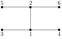
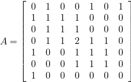
Example 3.11. LetGbe the graph shown in Figure 3.1. Gis the vertex sum of
s
3 s6
s
4
s
2 s5
s
1
s7
✧✧
✧✧
✧✧
❜ ❜
❜ ❜
❜ ❜
✧✧
✧
[image:15.595.223.358.517.602.2]❜ ❜ ❜
Fig. 3.1.A vertex sumGwithξ(G)greater than the maximum ofξon vertex summands
G1=1,2,3,4,5,6andG2 =1,7. HereWindicates the subgraph ofGinduced by the verticesW ⊂ {1,2, . . . , n}. Thenξ(G) = 3, because the matrix
A=
0 1 0 0 1 0 1
1 1 1 1 0 0 0
0 1 1 1 0 0 0
0 1 1 2 1 1 0
1 0 0 1 1 1 0
0 0 0 1 1 1 0
1 0 0 0 0 0 0
It is also interesting to contrast the behaviour of ξ and µ on clique sums. IfG
is a clique sum onKs ofGi, i= 1, . . . , kwith s <maxk
i=1µ(Gi) (as is the case for a vertex sum provided at least one Gi is not a path), then µ(G) = maxk
i=1µ(Gi) (see [10]).
In [10, Theorem 2.7] it is shown thatµ(G)µ(G−v) + 1, wherevis an arbitrary vertex in G, and if v is connected to every other vertex and G−v is connected of order greater than 1, then equality holds. Do the same results hold for ξ? We have some partial results.
Lemma 3.12. IfGis connected,|G|>1, andG′ is obtained by joiningv to each
vertex of G, then ξ(G′)ξ(G) + 1.
Proof. Let the new vertex be n. Choose a matrix A that is ξ-optimal for G,
so A ∈ S(G), corankA =ξ(G) and A has SAP. SinceG is connected and|G| >1, there is no column of Aconsisting entirely of 0’s. So there is a b∈R(A) such that every entrybi is nonzero. Since b∈R(A), there existsu∈Rn−1such that b=Au.
Let A′ = A Au
uTA uTAu
. Then rankA′ = rankA so corankA′ = corankA+ 1.
Sincebi= 0 for alli,A′ ∈ S(G′). LetX′ fully annihilateA′. Then X′ = X 0
0T 0
(since n is joined to every other vertex). In addition, A′X′ = 0 implies AX = 0,
and since A has SAP, we conclude X = 0, that is, X′ = 0. Thus A′ has SAP, so ξ(G′)corankA′= corankA+ 1 =ξ(G) + 1.
Lemma 3.13. If there exists aξ-optimalAforGwithb∈R(A(v)), thenξ(G) ξ(G−v) + 1.
Proof. Without loss of generality,v= 1. LetAbeξ-optimal forGwithb∈R(A0)
where A = α b
T
b A0
. Then by Lemma 3.5, A0 has SAP. rank A0 rankA, so
corankA0corankA−1 =ξ(G)−1. SinceA0 has SAP,ξ(G−v)corankA0. A graph G is calledvertex transitive if, for any two distinct vertices u, v of G, there is an automorphism (that is, a bijection fromV toV that preserves adjacency) ofGmappingutov.
Corollary 3.14. IfGis vertex transitive, then ξ(G)≤ξ(G−v) + 1.
Proof. Without loss of generality,v= 1. LetGbe vertex transitive and letAbe
ξ-optimal forG. SinceAis singular, there is a row, sayk, that is a linear combination of other rows of A. Since G is vertex transitive, there is a graph automorphism ψ
such thatψ(1) =k. LetPψ be the permutation matrix forψ, i.e., rowiofPψ is row
ψ(i) of the identity matrix. Then sinceψ is an automorphism ofG, PψAPT
ψ ∈ S(G)
and row 1 ofPψAPT
ψ is a linear combination of the other rows. Thus by Lemma 3.13, ξ(G)ξ(G−v) + 1.
If G and H are two graphs, then the join of G and H, denoted by G∨H, is the graph obtained from the disjoint union ofGandH by adding an edge from each vertex ofGto each vertex ofH.
Lemma 3.15. If G =G1∨G2, A ∈ S(G) is partitioned as A1 B
BT A
2
with
Proof. Suppose X fully annihilatesA. ThenX has the formX = X1 0 0T X
2
,
andAX= BA1TXX1 BX2
1 A2X2
= 0, so thatAiXi= 0 fori= 1,2. Since Ai has SAP,
Xi= 0 and Ahas SAP.
Theorem 3.16. If Gis connected,|G|>1 andξ(G) =M(G), then
ξ(G∨Kr) =ξ(G) +r=M(G∨Kr).
Proof. The graph G∨Kr can be obtained fromG by adjoining one vertex at a
time to all vertices of previous graph. By Lemma 3.12,ξ(G∨Kr)ξ(G) +r. Since
ξ(G) =M(G), ξ(G) = |G|−mr(G). Thus ξ(G) +r ξ(G∨Kr) M(G∨Kr) |G∨Kr| −mr(G∨Kr)|G|+r−mr(G) =ξ(G) +r.
Corollary 3.17. There is a graph on nvertices with minimum rank khaving
n(n−1)
2 −
k(k−1)
2 edges. This can be obtained as G=Pk+1∨Kn−k−1 or from Kn by
deleting k(k−21) (specific) edges. This graph satisfies ξ(G) =M(G).
REFERENCES
[1] F. Barioli and S. M. Fallat. On two conjectures regarding an inverse eigenvalue problem for acyclic symmetric matrices. Electronic Journal of Linear Algebra, 11:41–50, 2004. [2] F. Barioli, S. Fallat, and L. Hogben. Computation of minimal rankand path cover number for
graphs. Linear Algebra and its Applications, 392:289–303, 2004.
[3] F. Barioli, S. Fallat, and L. Hogben. On the difference between the maximum multiplicity and path cover number for tree-like graphs. Linear Algebra and its Applications, 409:13–31, 2005.
[4] W. W. Barrett, H. van der Holst, and R. Loewy. Graphs whose minimal rankis two.Electronic
Journal of Linear Algebra, 11:258–280, 2004.
[5] Y. Colin de Verdi`ere. On a new graph invariant and a criterion for planarity. InGraph Structure
Theory. Contemporary Mathematics 147, American Mathematical Society, Providence, pp.
137–147, 1993.
[6] Y. Colin de Verdi`ere. Multplicities of eigenvalues and tree-width graphs.Journal of
Combina-torial Theory, Series B, 74:121–146, 1998.
[7] R. Diestel Graph Theory. Springer-Verlag, New York, 1997. Electronic edition, 2000: http://www.math.uni-hamburg.de/home/diestel/books/graph.theory/download.html [8] M. Fiedler. A characterization of tridiagonal matrices. Linear Algebra and its Applications,
2:191–197, 1969.
[9] H. van der Holst. Topological and spectral graph characterizations. Ph. D. Thesis, University of Amsterdam, Amsterdam, 1996.
[10] H. van der Holst, L. Lov´asz, and A. Schrijver. The Colin de Verdi`ere graph parameter. In
Graph Theory and Computational Biology (Balatonlelle, 1996). Mathematical Studies,
Janos Bolyai Math. Soc., Budapest, pp. 29–85, 1999.
[11] C.R. Johnson and A. Leal Duarte. The maximum multiplicity of an eigenvalue in a matrix whose graph is a tree. Linear and Multilinear Algebra, 46:139–144, 1999.
[12] C.R. Johnson, A. Leal Duarte, and C. Saiago. The Parter-Wiener theorem: refinement and generalization SIAM Journal on Matrix Analysis and Applications, 25:352–361, 2003. [13] P.M. Nylen. Minimum-rankmatrices with prescribed graph. Linear Algebra and its
[14] S. Parter. On the eigenvalues and eigenvectors of a class of matrices. Journal of the Society
for Industrial and Applied Mathematics, 8:376–388, 1960.
[15] G. Wiener. Spectral multiplicity and splitting results for a class of qualitative matrices.Linear