q
-Deformed KP Hierarchy
and
q
-Deformed Constrained KP Hierarchy
Jingsong HE †‡, Yinghua LI † and Yi CHENG†
† Department of Mathematics, University of Science and Technology of China, Hefei,
230026 Anhui, P.R. China
E-mail: [email protected], [email protected]
‡ Centre for Scientific Computing, University of Warwick, Coventry CV4 7AL, United Kingdom
Received January 27, 2006, in final form April 28, 2006; Published online June 13, 2006 Original article is available athttp://www.emis.de/journals/SIGMA/2006/Paper060/
Abstract. Using the determinant representation of gauge transformation operator, we have shown that the general form ofτ function of theq-KP hierarchy is aq-deformed generalized Wronskian, which includes the q-deformed Wronskian as a special case. On the basis of these, we study theq-deformed constrained KP (q-cKP) hierarchy, i.e.l-constraints ofq-KP hierarchy. Similar to the ordinary constrained KP (cKP) hierarchy, a large class of solutions of q-cKP hierarchy can be represented byq-deformed Wronskian determinant of functions satisfying a set of linear q-partial differential equations with constant coefficients. We obtained additional conditions for these functions imposed by the constraints. In particular, the effects of q-deformation (q-effects) in single q-soliton from the simplest τ function of the q-KP hierarchy and in multi-q-soliton from one-component q-cKP hierarchy, and their dependence of xandq, were also presented. Finally, we observe that q-soliton tends to the usual soliton of the KP equation whenx→0 andq→1, simultaneously.
Key words: q-deformation; τ function; Gauge transformation operator; q-KP hierarchy; q-cKP hierarchy
2000 Mathematics Subject Classification: 37K10; 35Q51; 35Q53; 35Q55
1
Introduction
Study of the quantum calculus (or q-calculus) [1,2] has a long history, which may go back to the beginning of the twentieth century. F.H. Jackson was the first mathematician who studied theq-integral andq-derivative in a systematic way starting about 1910 [3,4]1. Since 1980’s, the
quantum calculus was re-discovered in the research of quantum group inspired by the studies on quantum integrable model that used the quantum inverse scattering method [5] and on noncommutative geometry [6]. In particular, S. Majid derived theq-derivative from the braided differential calculus [7,8].
The q-deformed integrable system (also called q-analogue or q-deformation of classical inte-grable system) is defined by means of q-derivative∂q instead of usual derivative ∂ with respect
to x in a classical system. It reduces to a classical integrable system as q → 1. Recently, the q-deformation of the following three stereotypes for integrable systems attracted more attention. The first type is q-deformedN-th KdV (q-NKdV orq-Gelfand–Dickey hierarchy) [9,16], which is reduced to the N-th KdV (NKdV or Gelfand–Dickey) hierarchy when q → 1. The N-th q-KdV hierarchy becomesq-KdV hierarchy forN = 2. Theq-NKdV hierarchy inherited several integrable structures from classicalN-th KdV hierarchy, such as infinite conservation laws [10],
1 Detailed notes on the initial research of
bi-Hamiltonian structure [11,12],τ function [13,14], B¨acklund transformation [15]. The second type is the q-KP hierarchy [17, 22]. Its τ function, bi-Hamiltonian structure and additional symmetries have already been reported in [20, 21, 18, 22]. The third type is the q-AKNS-D hierarchy, and its bilinear identity and τ function were obtained in [23].
In order to get the Darboux–B¨acklund transformations, the two elementary types of gauge transformation operators, differential-type denoted by T (or TD) and integral-type denoted
by S (or TI), for q-deformed N-th KdV hierarchy were introduced in [15]. Tu et al. obtained
not only the q-deformed Wronskian-type but also binary-type representations of τ function of q-KdV hierarchy. On the basis of their results, He et al. [24] obtained the determinant representation of gauge transformation operatorsTn+k (n≥k) forq-Gelfand–Dickey hierarchy,
which is a mixed iteration of n-steps of TD and then k-steps ofTI. Then, they obtained a more
general form of τ function for q-KdV hierarchy, i.e., generalized q-deformed Wronskian (q -Wronskian) IWnq+k [24]. It is important to note that for k = 0 IWnq+k reduces to q-deformed Wronskian and for k= n to binary-type determinant [15]. On the other hand, Tu introduced theq-deformed constrained KP (q-cKP) hierarchy [22] by means of symmetry constraint ofq-KP hierarchy, which is a q-analogue of constrained KP (cKP) hierarchy [25,31].
The purpose of this paper is to construct theτ function of q-KP andq-cKP hierarchy, and then explore theq-effect inq-solitons. The main tool is the determinant representation of gauge transformation operators [32, 33, 34, 35]. The paper is organized as follows: In Section 2 we introduce some basic facts on the q-KP hierarchy, such as Lax operator, Z-S equations, the existence of τ function. On the basis of the [15], two kinds of elementary gauge transformation operators for q-KP hierarchy and changing rule of q-KP hierarchy under it are presented in Section 3. In Section 4, we establish the determinant representation of gauge transformation operator Tn+k for the q-KP hierarchy and then obtain the general form of τ function τq(n+k) =
IWnq+k. In particular, by taking n= 1, k = 0 we will show q-effect of singleq-soliton solution of q-KP hierarchy. A brief description of the sub-hierarchy of q-cKP hierarchy is presented in Section 5, from the viewpoint of the symmetry constraint. In Section 6, we show that the q -Wronskian is one kind of forms ofτ function ofq-cKP if the functions in theq-Wronskian satisfy some restrictions. In Section 7 we consider an example which illustrates the procedure reducing q-KP to q-cKP hierarchy. q-effects of the q-deformed multi-soliton are also discussed. The conclusions and discussions are given in Section 8. Our presentation is similar to the relevant papers of classical KP and cKP hierarchy [32,34,36,37,38].
At the end of this section, we shall collect some useful formulae for reader’s convenience. Theq-derivative ∂q is defined by
∂q(f(x)) =
f(qx)−f(x) x(q−1)
and theq-shift operator is given by
θ(f(x)) =f(qx).
Let ∂−1
q denote the formal inverse of∂q. We should note that θ does not commute with∂q,
(∂qθk(f)) =qkθk(∂qf), k∈Z.
In general, the following q-deformed Leibnitz rule holds:
∂qn◦f =X
k≥0
n k
q
where the q-number and theq-binomial are defined by
(n)q=
qn−1
q−1 ,
n k
q
= (n)q(n−1)q· · ·(n−k+ 1)q (1)q(2)q· · ·(k)q
,
n 0
q
= 1,
and “◦” means composition of operators, defined by∂q◦f = (∂q·f) +θ(f)∂q. In the remainder
of the paper for any function f “·” is defined by ∂q ·f = ∂q(f) , (∂qf). For a q
-pseudo-differential operator (q-PDO) of the formP =
n
P
i=−∞
pi∂qi, we decompose P into the differential
part P+ = P
i≥0
pi∂qi and the integral partP− = P
i≤−1
pi∂qi. The conjugate operation “∗” for P is
defined byP∗ =P
i
(∂∗
q)ipi with∂q∗ =−∂qθ−1 =−1q∂1 q, (∂
−1
q )∗ = (∂q∗)−1 =−θ∂q−1. We can write
out several explicit forms of (1.1) for q-derivative∂q, as
∂q◦f = (∂qf) +θ(f)∂q, (1.2)
∂q2◦f = (∂q2f) + (q+ 1)θ(∂qf)∂q+θ2(f)∂q2, (1.3)
∂q3◦f = (∂q3f) + (q2+q+ 1)θ(∂q2f)∂q+ (q2+q+ 1)θ2(∂qf)∂2q+θ3(f)∂q3, (1.4)
and ∂−1
q
∂q−1◦f =θ−1(f)∂q−1−q−1θ−2(∂qf)∂q−2+q−3θ−3(∂q2f)∂q−3−q−6θ−4(∂q3f)∂q−4
+ 1 q10θ
−5(∂4
qf)∂q−5+· · ·+ (−1)kq−(1+2+3+···+k)θ−k−1(∂qkf)∂q−k−1+· · · , (1.5)
∂q−2◦f =θ−2(f)∂q−2− 1
q2(2)qθ −3(∂
qf)∂q−3+
1
q(2+3)(3)qθ −4(∂2
qf)∂q−4
− 1
q(2+3+4)(4)qθ −5(∂3
qf)∂q−5+· · ·
+ (−1)
k
q(2+3+···+k+1)(k+ 1)qθ
−2−k(∂k
qf)∂q−2−k+· · · . (1.6)
More explicit expressions of∂qn◦f are given in Appendix A. In particular,∂q−1◦f has different forms,
∂q−1◦f =θ−1(f)∂q−1+∂q−1◦(∂q∗f)◦∂q−1,
∂q−1◦f ◦∂q−1 = (∂q−1f)∂−q1−∂q−1◦θ(∂q−1f),
which will be used in the following sections. The q-exponent eq(x) is defined as follows
eq(x) =
∞
X
i=0 xn (n)q!
, (n)q! = (n)q(n−1)q(n−2)q· · ·(1)q.
Its equivalent expression is of the form
eq(x) = exp
∞
X
k=1
(1−q)k
k(1−qk)x k
!
. (1.7)
2
q
-KP hierarchy
Similarly to the general way of describing the classical KP hierarchy [36,37], we shall give a brief introduction of q-KP based on [20]. Let L be oneq-PDO given by
L=∂q+u0+u−1∂q−1+u−2∂q−2+· · · , (2.1)
which is called Lax operator of q-KP hierarchy. There exist infinite q-partial differential equa-tions relating to dynamical variables {ui(x, t1, t2, t3, . . .), i = 0,−1,−2,−3, . . .}, and they can
be deduced from generalized Lax equation,
∂L ∂tn
= [Bn, L], n= 1,2,3, . . . , (2.2)
which are calledq-KP hierarchy. HereBn= (Ln)+=
n
P
i=0
bi∂qi means the positive part ofq-PDO,
and we will use Ln− = Ln−Ln+ to denote the negative part. By means of the formulae given
in (1.2)–(1.6) and in Appendices A and B, the first few flows in (2.2) for dynamical variables
{u0, u−1, u−2, u−3}can be written out as follows. The first flow is
∂t1u0=θ(u−1)−u−1,
∂t1u−1= (∂qu−1) +θ(u−2) +u0u−1−u−2−u−1θ
−1(u 0),
∂t1u−2= (∂qu−2) +θ(u−3) +u0u−2−u−3−u−2θ
−2(u 0) +
1 qu−1θ
−2(∂
qu0),
∂t1u−3= (∂qu−3) +θ(u−4) +u0u−3−u−4− 1 q3u−1θ
−3(∂2
qu0)
+ 1
q2(2)qu−2θ −3(∂
qu0)−u−3θ−3(u0).
The second flow is
∂t2u0=θ(∂qu−1) +θ
2(u
−2) +θ(u0)θ(u−1) +u0θ(u−1)
− (∂qu−1) +u−1u0+u−1θ−1(u0) +u−2, ∂t2u−1=q
−1u
−1θ−2(∂qu0) +u−1(∂qu0) + (∂q2u−1) + θ(u0) +u0(∂qu−1)
+ (q+ 1)θ(∂qu−2) +θ(u0)θ(u−2) +u0θ(u−2) +θ(u−1)u−1+u20u−1
−u−1θ−1(u20)−u−1θ−1(u−1)−u−2θ−1(u0)−u−2θ−2(u0) +θ3(u−3)−u−3, ∂t2u−2= (∂
2
qu−2) + (q+ 1)θ(∂qu−3) + (∂qu−2)v1+θ2(u−4) +θ(u−3)v1+u−2v0
− q−3u−1θ−3(∂q2v1)−q−1u−1θ−2(∂qv0)−q−2(2)qu−2θ−3(∂qv1)
+u−2θ−2(v0) +u−3θ−3(v1) +u−4, ∂t2u−3= (∂
2
qu−3) + (q+ 1)θ(∂qu−4) + (∂qu−3)v1+θ2(u−5) +θ(u−4)v1+u−3v0
− −q−6θ−4(∂3qv1) +q−3u−1θ−3(∂q2v0) +q−5(3)qu−2θ−4(∂q2v1)
−q−2(2)qu−2θ−3(∂qv0)−q−3(3)qu−3θ−4(∂qv1) +u−3θ−3(v0)
+u−4θ−4(v1) +u−5.
The third flow is
∂t3u0= (∂
3
qu0) + (3)qθ(∂2qu−1) + ˜s2(∂q2u0) + (3)qθ2(∂qu−2) + (2)qθ(∂qu−1)˜s2
+ (∂qu0)˜s1+θ3(u−3) +θ2(u−2)˜s2+θ(u−1)˜s1+u0s˜0
∂t3u−1= (∂
3
qu−1) + (3)qθ(∂q2u−2) + ˜s2(∂q2u−1) + (3)qθ2(∂qu−3) + (2)qs˜2θ(∂qu−2)
+ ˜s1(∂qu−1) +θ3(u−4) + ˜s2θ3(u−3) + ˜s1θ(u−2) + ˜s0u−1
− q−3u−1θ−3(∂q2s˜2)−q−1u−1θ−2(∂qs˜1)−q−2(2)qu−2θ−3(∂qs˜2)
+u−1θ−1(˜s0) +u−2θ−2(˜s1) +u−3θ−3(˜s2) +u−4,
∂t3u−2= (∂
3
qu−2) + (3)qθ(∂q2u−3) + ˜s2(∂q2u−2) + (3)qθ2(∂qu−4) + (2)qs˜2θ(∂qu−3)
+ ˜s1(∂qu−2) +θ3(u−5) + ˜s2θ2(u−4) + ˜s1θ(u−3) + ˜s0u−2
− −q−6u−1θ−4(∂q3s˜2) +q−3u−1θ−3(∂q2s˜1) +q−5(3)qu−2θ−4(∂q2˜s2)
−q−1u−1θ−2(∂qs˜0)−q−2(2)qu−2θ−3(∂qs˜1)−q−3(3)qu−3θ−4(∂q˜s2)
+u−2θ−2(˜s0) +u−3θ−3(˜s1) +u−4θ−4(˜s2) +u−5,
∂t3u−3= (∂
2
qu−3) + (3)qθ(∂q2u−4) + ˜s2(∂q2u−3) + (3)qθ2(∂qu−5) + (2)qs˜2θ(∂qu−4)
+ ˜s1(∂qu−3) +θ3(u−6) + ˜s2θ2(u−5) + ˜s1θ(u−4) + ˜s0u−3
− q−10u−1θ−5(∂q4s˜2)−q−6u−1θ−4(∂q3˜s1)−q−9(4)qθ−5(∂q3˜s2)
+q−3u−1θ−3(∂q2s˜0) +q−5(3)qu−2θ−4(∂q2˜s1) +q−7
(3)q(4)4
(2)q
u−3θ−5(∂2q˜s2)
−q−2(2)
qu−2θ−3(∂qs˜0)−q−3(3)qu−3θ−4(∂qs˜1)−q−4(4)qu−4θ−5(∂qs˜2)
+u−3θ−3(˜s0) +u−4θ−4(˜s1) +u−5θ−5(˜s2) +u−6.
Obviously,∂t1 =∂ and equations of flows here are reduced to usual KP flows (4.10) and (4.11) in [39] when q→1 and u0 = 0. If we only consider the first three flows, i.e. flows of (t1, t2, t3),
then u−1=u−1(t1, t2, t3) is a q-deformation of the solution of KP equation [39]
∂ ∂t1
4∂u
∂t3
−12u∂u ∂t1
−∂
3u
∂t3 1
−3∂
2u
∂t2 2
= 0.
In other words, u−1 = u(t1, t2, t3) in the above equation when q → 1, and hence u−1 is called
a q-soliton ifu(t1, t2, t3) = lim
q→1u−1 is a soliton solution of KP equation.
On the other hand, L in (2.1) can be generated by dressing operator S = 1 + P∞
k=1
sk∂q−k in
the following way
L=S◦∂q◦S−1. (2.3)
Further, the dressing operatorS satisfies the Sato equation
∂S ∂tn
=−(Ln)−S, n= 1,2,3, . . . . (2.4)
Theq-wave functionwq(x, t) andq-adjoint wave functionw∗q(x, t) forq-KP hierarchy are defined
by
wq(x, t;z) = Seq(xz) exp
∞
X
i=1 tizi
!!
(2.5)
and
w∗(x, t;z) = (S∗)−1|x/qe1/q(−xz) exp −
∞
X
i=1 tizi
!!
where t= (t1, t2, t3, . . .). Here, for aq-PDOP =P
i
pi(x)∂iq, the notation
P|x/t =
X
i
pi(x/t)ti∂qi
is used in (2.6). Note that wq(x, t) and wq∗(x, t) satisfy following linearq-differential equations,
(Lwq) =zwq,
∂wq
∂tn = (Bnwq),
(L∗|
x/qwq∗) =zwq∗,
∂w∗
q
∂tn
=−((Bn|x/q)∗w∗q). (2.7)
Furthermore, wq(x, t) and wq∗(x, t) can be expressed by sole functionτq(x, t) as
ωq =
τq(x;t−[z−1])
τq(x;t)
eq(xz) exp
∞
X
i=1 tizi
!
, (2.8)
ωq∗ = τq(x;t+ [z
−1])
τq(x;t)
e1/q(−xz) exp −
∞
X
i=1 tizi
! ,
where
[z] =
z,z 2
2 , z3
3, . . .
.
From comparison of (2.5) and (2.8), the dressing operatorS has the form of
S = 1−
1 τq
∂ ∂t1
τq
∂q−1+
1 2τq
∂2 ∂t2
1
− ∂
∂t2
τq
∂q−2+· · · . (2.9)
Using (2.9) in (2.3), and then comparing with Lax operator in (2.1), we can show that all dynamical variablesui (i= 0,−1,−2,−3, . . .) can be expressed byτq(x, t), and the first two are
u0=s1−θ(s1) =−x(q−1)∂qs1=x(q−1)∂q∂t1lnτq,
u−1 =−∂qs1+s2−θ(s2) +θ(s1)s1−s21, (2.10)
· · · ·
We can see u0 = 0, and u−1 = (∂x2logτ) as classical KP hierarchy when q → 1, where τ =
τq(x, t)|q→1. By considering u−1 depending only on (q, x, t1, t2, t3), we can regard u−1 as q
-deformation of solution of classical KP equation. We shall show the q-effect of this solution for q-KP hierarchy after we get τq in next section. In order to guarantee thateq(x) is convergent,
we require the parameter 0< q <1 and parameterx to be bounded.
Beside existence of the Lax operator,q-wave function,τq forq-KP hierarchy, another
impor-tant property is the q-deformed Z-S equation and associated linear q-differential equation. In other words, q-KP hierarchy also has an alternative expression, i.e.,
∂Bm
∂tn
− ∂Bn
∂tm
+ [Bm, Bn] = 0, m, n= 1,2,3, . . . . (2.11)
The “eigenfunction”φand “adjoint eigenfunction”ψ ofq-KP hierarchy associated to (2.11) are defined by
∂φ ∂tn
= (Bnφ), (2.12)
∂ψ ∂tn
=−(Bn∗ψ), (2.13)
3
Gauge transformations of
q
-KP hierarchy
The authors in [15] reported two types of elementary gauge transformation operator only forq -Gelfand–Dickey hierarchy. We extended the elementary gauge transformations given in [15], for theq-KP hierarchy. At the same time, we shall add some vital operator identity concerning to the q-differential operator and its inverse. Here we shall prove two transforming rules ofτ function, “eigenfunction” and “adjoint eigenfunction” of theq-KP hierarchy under these transformations. Majority of the proofs are similar to the classical case given by [32,33] and [35], so we will omit part of the proofs.
SupposeT is a pseudo-differential operator, and
L(1) =T ◦L◦T−1, Bn(1) ≡ L(1)n+,
so that
∂ ∂tn
L(1)=Bn(1), L(1)
still holds for the transformed Lax operatorL(1); thenTis called a gauge transformation operator of the q-KP hierarchy.
Lemma 1. The operator T is a gauge transformation operator, if
T◦Bn◦T−1+=T ◦Bn◦T−1+ ∂T
∂tn
◦T−1, (3.1)
or
T◦Bn◦T−1−=−
∂T ∂tn
◦T−1. (3.2)
If the initial Lax operator ofq-KP is a “free” operatorL=∂q, then the gauge transformation
operator is also a dressing operator for new q-KP hierarchy whose Lax operator L(1)=T ◦∂q◦
T−1, because of (3.2) becomes
Ttn =− T◦Bn◦T
−1
−◦T =− T◦∂
n q ◦T−1
−◦T =− L (1)n
−◦T, (3.3)
which is the Sato equation (2.4). In order to prove existence of two types of the gauge transfor-mation operator, the following operator identities are necessary.
Lemma 2. Let f be a suitable function, and A be a q-deformed pseudo-differential operator, then
(1) θ(f)◦∂q◦f−1◦A◦f ◦∂q−1◦(θ(f))−1
+
=θ(f)◦∂q◦f−1◦A+◦f◦∂q−1◦(θ(f))−1
−θ(f)◦∂q f−1·(A+·f)◦∂q−1◦(θ(f))−1, (3.4)
(2) θ−1(f−1)◦∂q−1◦f ◦A◦f−1◦∂q◦θ−1(f)−
=θ−1(f−1)◦∂q−1◦f ◦A−◦f−1◦∂q◦θ−1(f)
−θ−1(f−1)◦∂q−1◦θ−1(f)◦∂q θ−1[f−1· A∗+·f
]. (3.5)
Theorem 1. There exist two kinds of gauge transformation operator for the q-KP hierarchy, namely
Type I : TD(φ1) =θ(φ1)◦∂q◦φ−11, (3.6)
Type II : TI(ψ1) = (θ−1(ψ1))−1◦∂q−1◦ψ1. (3.7)
Here φ1 andψ1 are defined by (2.12)and (2.13) that are called the generating functions of gauge transformation.
Proof . First of all, for the Type I case (see (3.6)),
B(1)n ≡ L(1)n+= TD◦(L)n◦TD−1+
=TD◦Bn◦TD−1−θ(φ1)·∂q φ1−1·(Bn·φ1)◦∂q−1◦(θ(φ1))−1
=TD◦Bn(0)◦TD−1−
θ(φ1)◦∂q◦
(φ1)tn φ1
◦∂q−1◦(θ(φ1))−1
−θ(φ1)◦θ (φ1)t
n φ1
◦∂q◦∂q−1◦(θ(φ1))−1
=TD◦Bn◦TD−1+θ
(φ1)t n φ1
−θ(φ1)◦∂q◦
(φ1)tn φ1
◦∂q−1◦(θ(φ1))−1.
Here the operator identity (3.4), Bn = (L)n+, (φ1)tn = (Bn·φ1) and (1.2) were used. On the other hand,
∂TD
∂tn
◦TD−1= θ(φ1)◦∂q◦φ−11
tn◦T
−1
D =θ((φ1)tn)◦∂q◦φ
−1
1 ◦φ1◦∂−q1◦(θ(φ1))−1
−θ(φ1)◦∂q◦
(φ1)tn
φ21 ◦φ1◦∂
−1
q ◦(θ(φ1))−1
=θ(φ1)tn φ1
−θ(φ1)◦∂q◦
(φ1)tn φ1
◦∂q−1◦(θ(φ1))−1.
Taking this expression back into Bn(1), we get
B(1)n ≡ L(1)n+=TD◦Bn◦TD−1+
∂TD
∂tn
◦TD−1,
and that indicates that TD(φ1) is indeed a gauge transformation operator via Lemma1. Second,
we want to prove that the equation (3.2) holds for Type II case (see (3.7)). By direct calculation the left hand side of (3.2) is in the form of
TI◦Bn◦TI−1−= (θ−1(ψ1))−1◦∂q−1◦ψ1◦Bn◦ψ1−1◦∂q◦θ−1(ψ1)−
= (θ−1(ψ1))−1◦∂q−1◦ψ1◦(Bn)−◦ψ1−1◦∂q◦θ−1(ψ1)
−(θ−1(ψ1))−1◦∂q−1◦θ−1(ψ1)◦ ∂qθ−1
B∗
n·ψ1 ψ1
!!
= (θ−1(ψ1))−1◦∂q−1◦θ−1(ψ1)◦ ∂qθ−1
ψ1tn ψ1
!! .
In the above calculation, the operator identity (3.5), (Bn)−= 0, (ψ1)tn =−(B
∗
n·ψ1) were used.
Moreover, with the help of (1.2), we have
−∂TI
∂tn
◦TI−1 =− ∂
∂tn
(θ−1(ψ
= θ
−1((ψ 1)tn) (θ−1(ψ
1))2
◦∂q−1◦ψ1◦ψ1−1◦∂q◦θ−1(ψ1)
−(θ−1(ψ1))−1◦∂q−1◦(ψ1)tn◦ψ
−1
1 ◦∂q◦θ−1(ψ1)
=θ−1
(ψ1)tn ψ1
− 1
θ−1(ψ 1)
◦∂q−1◦
∂q◦θ−1
(ψ1)tn
ψ1
−
∂q·θ−1
(ψ1)tn
ψ1
◦θ−1(ψ1) =θ−1
(ψ1)tn ψ1
−θ−1
(ψ1)tn ψ1
+ 1
θ−1(ψ 1)
◦∂q−1◦
∂q·θ−1
(ψ1)tn
ψ1
◦θ−1(ψ1)
= 1
θ−1(ψ 1)
◦∂q−1◦
∂q·θ−1
(ψ1)tn
ψ1
◦θ−1(ψ1).
The two equations obtained above show that TI(ψ1) satisfies (3.2), so TI(ψ1) is also a gauge
transformation operator of the q-KP hierarchy according to Lemma1.
Remark 2. There are two convenient expressions for TD and TI,
TD =∂q−α1, TD−1 =∂q−1+θ−1(α1)∂q−2+· · · , α1 = ∂qφ1
φ1
, (3.8)
TI= (∂q+β1)−1 =∂q−1−θ−1(β1)∂q−2+· · · , β1 =
∂qθ−1(ψ1) ψ1
. (3.9)
In order to get a new solution of q-KP hierarchy from the input solution, we should know the transformed expressions of u(1)i , τq(1),φ(1)i ,ψi(1). The following two theorems are related to
this. Before we start to discuss explicit forms of them, we would like to define the generalized q-Wronskian for a set of functions {ψk, ψk−1, . . . , ψ1;φ1, φ2, . . . , φn } as
IWk,nq (ψk, . . . , ψ1;φ1, . . . , φn) =
∂−1
q ψkφ1 ∂q−1ψkφ2 · · · ∂q−1ψkφn
..
. ... · · · ...
∂−1
q ψ1φ1 ∂q−1ψ1φ2 · · · ∂q−1ψ1φn
φ1 φ2 · · · φn
∂qφ1 ∂qφ2 · · · ∂qφn
..
. ... · · · ...
∂n−k−1
q φ1 ∂qn−k−1φ2 · · · ∂qn−k−1φn
,
which reduce to theq-Wronskian when k= 0,
Wnq(φ1,· · · , φn) =
φ1 φ2 · · · φn
∂qφ1 ∂qφ2 · · · ∂qφn
..
. ... · · · ...
∂n−1
q φ1 ∂qn−1φ2 · · · ∂qn−1φn
.
Suppose φ1(λ1;x, t) is a known “eigenfunction” of q-KP with the initial function τq, which
generates gauge transformation operator TD(φ1). Then we have
Theorem 2. Under the gauge transformationL(1)=T
D(φ1)◦L◦(TD(φ1))−1, new “eigenfunc-tion”, “adjoint eigenfunction” and τ function of the transformed q-KP hierarchy are
φ−→φ(1)(λ;x, t) = (TD(φ1)·φ) =
W2q(φ1, φ) φ1
ψ−→ψ(1)(λ;x, t) = TD(φ1)−1∗·ψ= θ(∂−1
q φ1ψ) θ(φ1)
,
τq −→τq(1)=φ1τq.
φ(1)k =φ(1)(λ=λk;x, t), ψk(1)=ψ(1)(λ=λk;x, t). Note φ(1)1 = 0.
Proof . (1) By direct calculations, we have
∂tnφ
(1)= (∂
tn(TD ·φ)) = (∂tnTD)·φ+ (TD·∂tnφ)
= ∂tnTD◦T
−1
D
·(TDφ) +TD ·(Bnφ) = ∂tnTD◦T
−1
D +TD◦Bn◦TD−1
·(TDφ)
= Bn(1)·φ(1),
in which (2.12) and (3.1) were used.
(2) Similarly, with the help of (Bn(1))∗ = (TD−1)∗◦∂tnT
∗
D+ (TD−1)∗◦Bn∗◦TD∗ and (2.13), we
can obtain
∂tnψ
(1) = (T−1
D )∗·ψ
tn = −(T
∗
D)−1◦∂tnT
∗
D ◦(TD∗)−1
·ψ+ (TD∗)−1·∂tnψ
=− (TD−1)∗◦∂tnT
∗
D + (TD−1)∗◦Bn∗ ◦TD∗
· (TD−1)∗·ψ=− Bn(1)∗·ψ(1).
(3) According to the definition ofTD in (3.6) and with the help of (3.8),L(1) can be expressed
as
L(1)q =∂q+u(1)0 +u (1)
−1∂q−1+· · ·, u(1)0 =x(q−1)∂qα1+θ(u0).
On the other hand, (φ1)t1 = ((L)+φ1) impliesα1 =∂t1lnφ1−u0, thenu
(1)
0 becomes
u(1)0 =x(q−1)∂q∂t1lnφ1+u0=x(q−1)∂q∂t1lnφ1+x(q−1)∂q∂t1lnτq
=x(q−1)∂q∂t1lnφ1τq.
Then
τq(1) =φ1τq.
This completes the proof of the theorem.
For the gauge transformation operator of Type II, there exist similar results. Letψ1(µ1;x, t)
be a known “adjoint eigenfunction” of q-KP with the initial function τq, which generates the
gauge transformation operator TI(ψ1). Then we have
Theorem 3. Under the gauge transformationL(1)=TI(ψ1)◦L◦(TI(ψ1))−1, new “eigenfunc-tion”, “adjoint eigenfunction” and τ function of the transformed q-KP hierarchy are
φ−→φ(1)(λ;x, t) = (TI(ψ1)·φ) =
(∂−1
q ψ1φ) θ−1(ψ
1) ,
ψ−→ψ(1)(λ;x, t) = TI(ψ1)−1∗·ψ= f
W2q(ψ1, ψ) ψ1
,
τq −→τq(1)=θ−1(ψ1)τq.
φ(1)k =φ(1)(λ=λk;x, t), ψ(1)k =ψ(1)(λ=λk;x, t). Note ψ1(1) = 0. Wf
q
n is obtained from Wnq by
replacing ∂q with ∂∗q.
4
Successive applications of gauge transformations
We now discuss successive applications of the two types of gauge transformation operators in a general way, which is similar to the classical case [32, 34,35]. For example, consider the chain of gauge transformation operators,
L T (1) D φ1
−−−−−−→L(1) T (2) D φ
(1) 2
−−−−−−−→L(2) T (3) D φ
(2) 3
−−−−−−−→L(3) −→ · · · −→L(n−1) T (n) D φ
(n−1)
n
−−−−−−−−→L(n)
TI(n+1) ψ1
−−−−−−−→L(n+1) T (n+2)
I ψ
(n+1) 2
−−−−−−−−−−→L(n+2) −→ · · · −→L(n+k−1) T (n+k)
I ψ
(n+k−1)
k
−−−−−−−−−−−−→L(n+k). (4.1)
Here the index “i“ in a gauge transformation operator means the i-th gauge transformation, and φ(ij) (orψ(ij)) is transformed byj-steps gauge transformations from φi (orψi),L(i) is
trans-formed byj-step gauge transformations from the initial Lax operatorL. Successive applications of gauge transformation operator in (4.1) can be represented by
Tn+k =TI(n+k) ψk(n+k−1)· · ·TI(n+2) ψ(2n+1)
◦TI(n+1) ψ1(n)
◦TD(n) φ(nn−1)· · ·TD(2) φ(1)2 ◦TD(1)(φ1).
Our goal is to obtain φ(n+k), ψ(n+k), τq(n+k) of L(n+k) transformed from L by the Tn+k in the
above chain. All of these are based on the determinant representation of gauge transformation operator Tn+k. As the proof of the determinant representation ofTn+k is similar extremely to
the case of classical KP hierarchy [34], we will omit it.
Lemma 3. The gauge transformation operator Tn+k has the following determinant
representa-tion (n > k):
Tn+k =
1
IWk,nq (ψk, . . . , ψ1;φ1, . . . , φn)
∂−1
q ψkφ1 · · · ∂q−1ψkφn ∂−q1◦ψk
..
. · · · ... ...
∂−1
q ψ1φ1 · · · ∂q−1ψ1φn ∂q−1◦ψ1
φ1 · · · φn 1
∂qφ1 · · · ∂qφn ∂q
..
. · · · ... ...
∂n−k
q φ1 · · · ∂qn−kφn ∂qn−k
and
Tn−+1k =
φ1◦∂q−1 θ(∂q−1ψkφ1) · · · θ(∂q−1ψ1φ1) θ(φ1) · · · θ(∂qn−k−2φ1) φ2◦∂q−1 θ(∂q−1ψkφ2) · · · θ(∂q−1ψ1φ2) θ(φ2) · · · θ(∂qn−k−2φ2)
..
. ... · · · ... ... · · · ...
φn◦∂q−1 θ(∂q−1ψkφn) · · · θ(∂q−1ψ1φn) θ(φn) · · · θ(∂qn−k−2φn)
× (−1)
n−1
θ(IWk,nq (ψk, . . . , ψ1;φ1, . . . , φn)
.
Lemma 4. Under the case of n=k, Tn+k is given by
Tn+n=
1
IWn,nq (ψn, . . . , ψ1;φ1, . . . , φn)
∂−1
q ψnφ1 · · · ∂−q1ψnφn ∂q−1◦ψn
..
. · · · ... ...
∂−1
q ψ1φ1 · · · ∂q−1ψ1φn ∂q−1◦ψ1
φ1 · · · φn 1
but Tn−+1n becomes
Tn−+1n=
−1 ψn · · · ψ1
φ1◦∂q−1 θ(∂q−1ψnφ1) · · · θ(∂−q1ψ1φ1) ..
. ... · · · ...
φn◦∂q−1 θ(∂q−1ψnφn) · · · θ(∂q−1ψ1φn)
(−1)
θ(IWn,nq (ψn, . . . , ψ1;φ1, . . . , φn)
.
In the above lemmas,Tn+k are expanded with respect to the last column collecting all
sub-determinants on the left of the symbols ∂qi (i=−1,0,1,2, . . . , n−k); Tn−+1k are expanded with respect to the first column by means of collection of all minors on the right ofφi∂q−1. Basing on
the determinant representation, first of all, we would like to consider the case of k= 0 in (4.1), i.e.
L T (1) D φ1
−−−−−−→L(1) T (2) D φ
(1) 2
−−−−−−−→L(2) T (3) D φ
(2) 3
−−−−−−−→L(3) −→ · · · −→L(n−1) T (n) D φ
(n−1)
n
−−−−−−−−→L(n),
whose corresponding equivalent gauge transformation operator is
Tn=TD(n) φ(nn−1)
· · ·TD(2) φ(1)2 ◦TD(1)(φ1). (4.2)
Theorem 4. Under the gauge transformation Tn (n≥1),
φ(n)(λ;x, t) = (Tn·φ) =
Wnq+1(φ1, . . . , φn, φ)
Wnq(φ1, . . . , φn)
, (4.3)
ψ(n)(µ;x, t) = Tn−1∗·ψ= (−1)nθ IW
q
1,n(ψ;φ1, . . . , φn)
Wnq(φ1, . . . , φn)
!
, (4.4)
τq(n)=Wnq(φ1, . . . , φn)·τq.
Furthermore, φ(in) = φ(n)(λ = λi;x, t), ψi(n) = ψ(n)(µ = µi;x, t). Note φ(in) = 0 if i ∈ {1,2, . . . , n}.
Proof . (1) Successive application of Theorem2 implies
φ(n)=TD(n) φn(n−1)φ(n−1)=TD(n) φ(nn−1)TD(n−1) φn(n−−12)φ(n−2) =· · ·
=TD(n) φn(n−1)· · ·TD(2) φ(1)2 ◦TD(1)(φ1)φ= (Tn·φ).
Using the determinant representation ofTn in it leads toφ(n). Here TD(1)(φ1) =TD(φ1).
(2) Similarly, according to Theorem2 we have
ψ(n)= TD(n)−1∗ψ(n−1)= TD(n)−1∗ TD(n−1)−1∗ψ(n−2) =· · ·
= TD(n)−1∗ TD(n−1)−1∗· · · TD(3)−1∗ TD(2)−1∗ TD−1∗·ψ= Tn−1∗·ψ.
Thenψ(n) can be deduced by using the determinant representation ofT−1
n in the Lemma3with
k= 0. Here we omit the generating functions inTD(i)(i= 1,2, . . . , n), which are the same as (1). (3) Meanwhile, we can getτ(n) by repeated iteration according to the rule in Theorem 2,
τq(n)=φ(nn−1)τq(n−1) =φn(n−1)φn(n−−12)τq(n−2) =φ(nn−1)φ(nn−−12)φ(nn−−23)τq(n−3)=· · ·
=φ(nn−1)φn(n−−12)φ(nn−−23)· · ·φ(3)4 φ(2)3 φ(1)2 φ1τq
= W
q
n(φ1, φ2, φ3, . . . , φn)
Wnq−1(φ1, φ2, φ3, . . . , φn−1)
Wnq−1(φ1, φ2, φ3, . . . , φn−1) Wnq−2(φ1, φ2, φ3, . . . , φn−2)
Wnq−2(φ1, φ2, φ3, . . . , φn−2) Wnq−3(φ1, φ2, φ3, . . . , φn−3)
· · ·W q
4(φ1, φ2, φ3, φ4) W3q(φ1, φ2, φ3)
W3q(φ1, φ2, φ3) W2q(φ1, φ2)
W2q(φ1, φ2) W1q(φ1)
φ1τq =Wnq(φ1, φ2, . . . , φn)τq.
It should be noted that there is a θ action in (4.4), which is the main difference between the q-KP and classical KP beside different elements in determinant. Furthermore, for more complicated chain of gauge transformation operators in (4.1), φ(n+k),ψ(n+k), τq(n+k) of L(n+k)
can be expressed by the generalizedq-Wronskian.
Theorem 5. Under the gauge transformation Tn+k (n > k >0),
φ(n+k)(λ;x, t) = (Tn+k·φ) =
IWk,nq +1(ψk, . . . , ψ1;φ1, . . . , φn, φ)
IWk,nq (ψk, . . . , ψ1;φ1, . . . , φn)
,
ψ(n+k)(µ;x, t) = Tn−+1k∗·ψ= (−1)nIW
q
k+1,n(ψ, ψk, ψk−1, . . . , ψ1;φ1, . . . , φn)
IWk,nq (ψk, . . . , ψ1;φ1, . . . , φn)
,
τq(n+k)=IWk,nq (ψk, . . . , ψ1;φ1,· · · , φn)·τq.
Furthermore, φ(in+k) = φ(n+k)(λ = λ
i;x, t); ψi(n+k) = ψ(n+k)(µ = µi;x, t). Note φ(in+k) = 0 if
i∈ {1,2, . . . , n}, ψi(n+k)= 0 if i∈ {1,2, . . . , k}.
Proof . (1) The repeated iteration of Theorems2and3 according to the ordering ofTI andTD
deduces
φ(n+k) =TI(n+k) ψn(n++kk−1)·φ(n+k−1)
=TI(n+k) ψn(n++kk−1)TI(n+k−1) ψ(nn++kk−−12)·φ(n+k−2) =· · ·
=TI(n+k) ψn(n++kk−1)TI(n+k−1) ψn(n++kk−−12)· · ·TI(n+2) ψn(n+2+1)TI(n+1) ψ(nn+1) ·φ(n).
Then taking in it φ(n) = (T
n·φ) from (4.3) , we get
φ(n+k) = TI(n+k) ψn(n++kk−1)TI(n+k−1) ψn(n++kk−−12)· · ·TI(n+2) ψn(n+2+1)TI(n+1) ψn(n+1) Tn·φ
= (Tn+k·φ).
Therefore the determinant form ofφ(n+k) is given by Lemma3.
(2) Using Theorems 2 and 3 iteratively according to the chain in (4.1), similarly to the step (1), we can get
ψ(n+k)= TI(n+k)−1∗·ψ(n+k−1)= TI(n+k)−1∗ TI(n+k−1)−1∗·ψ(n+k−2) =· · ·
= TI(n+k)−1∗ TI(n+k−1)−1∗· · · TI(n+2)−1∗ TI(n+1)−1∗·ψ(n).
Noting that ψ(n) is given by (4.4), we getψ(n+k)= ((T−1
n+k)∗·ψ).The explicit form of ψ(n+k) is
given from the determinant representation of Tn−+1k.
(3) According to the changing rule under gauge transformation in Theorems2and3, the new τ function ofq-KP hierarchy τq(n+k) produced by chain of gauge transformations in (4.1) is
τq(n+k)=θ−1 ψk(n+k−1)τq(n+k−1) =θ−1 ψk(n+k−1)θ−1 ψk(n−+1k−2)τq(n+k−2)
=θ−1 ψk(n+k−1)θ−1 ψk(n−+1k−2)· · ·θ−1 ψ2(n+1)θ−1 ψ1(n)τq(n).
So the explicit form ofψ(in+i−1) (i= 1,2, . . . , k) andτq(n) implies
τq(n+k)= (−1)nIW
q
k,n(ψk, ψk−1, . . . , ψ1;φ1, φ2, . . . , φn)
×(−1)nIW
q
k−1,n(ψk−1, ψk−1, . . . , ψ1;φ1, φ2, . . . , φn)
IWkq−2,n(ψk−2, . . . , ψ1;φ1, φ2, . . . , φn)
· · ·(−1)nIW
q
2,n(ψ2, ψ1;φ1, φ2, . . . , φn)
IW1q,n(ψ1;φ1, φ2, . . . , φn)
×(−1)nIW
q
1,n(ψ1;φ1, φ2, . . . , φn)
Wnq(φ1, φ2, . . . , φn)
Wnq(φ1, φ2, . . . , φn)τq
≈IWk,nq (ψk, ψk−1, . . . , ψ1;φ1, φ2, . . . , φn)τq.
We omitted the trivial factor (−1)n in the last step, because it will not affect ui in the q-KP
hierarchy.
Remark 3. There exists another complicated chain of gauge transformation operators forq-KP hierarchy (that may be regarded as motivated by the classical KP hierarchy)
L T (1) I ψ1
−−−−−−→L(1) T (2) I ψ
(1) 2
−−−−−−−→L(2) T (3) I ψ
(2) 3
−−−−−−−→L(3) −→ · · · −→L(n−1) T (n) I ψ
(n−1)
n
−−−−−−−−−→L(n)
TD(n+1) φ(1n)
−−−−−−−−→L(n+1) T (n+2)
D φ
(n+1) 2
−−−−−−−−−−→L(n+2) −→ · · · −→L(n+k−1) T (n+k)
D φ
(n+k−1)
k
−−−−−−−−−−−−→L(n+k),
that can lead to another form of τq(n+k). This is parallel to the classical case of [32].
If the initialq-KP is a “free” operator, thenL=∂q that means the initialτ function is 1. We
can write down the explicit form of q-KP hierarchy generated by Tn+k. Under this situation,
(2.12) and (2.13) become
∂φ ∂tn
= (∂nqφ), ∂ψ ∂tn
=−(∂qn∗ψ), (4.5)
that possess set of solution {φi, ψi} as follows
φi(x;t) =eq(λi1x)e ∞
P
j=1
tjλji1
+aieq(µi1x)e ∞
P
j=1
tjµji1
, (4.6)
ψi(x;t) =e1/q(−λi2qx)e
−
∞
P
j=1
tjλji2
+bie1/q(−µi2qx)e
−
∞
P
j=1
tjµji2
. (4.7)
After the (n+k)-th step gauge transformationTn+k, the final form ofτqcan be given in following
corollary, which can be deduced directly from Theorems 4and 5.
Corollary 1. The gauge transformation can generate the following two forms ofτ function of the q-KP hierarchy,
τq(n+k)=IWk,nq (ψk, . . . , ψ1;φ1, . . . , φn) =
∂−1
q ψkφ1 ∂q−1ψkφ2 · · · ∂q−1ψkφn
..
. ... · · · ...
∂−1
q ψ1φ1 ∂q−1ψ1φ2 · · · ∂q−1ψ1φn
φ1 φ2 · · · φn
∂qφ1 ∂qφ2 · · · ∂qφn
..
. ... · · · ...
∂n−k−1
q φ1 ∂qn−k−1φ2 · · · ∂qn−k−1φn
,
τq(n)=Wnq(φ1, . . . , φn) =
φ1 φ2 · · · φn
∂qφ1 ∂qφ2 · · · ∂qφn
..
. ... · · · ...
∂n−1
q φ1 ∂qn−1φ2 · · · ∂qn−1φn
. (4.8)
On the other hand, we know from (3.3) thatTn defined by (4.2) is a dressing operator if its
generating functions are given by (4.6). Therefore we can define one q-wave function
ωq =Tn∂q−neq(xz)e
∞
P
i=1
zit i
= 1
Wnq
φ1 · · · φn z−n
∂qφ1 · · · ∂qφn z−n+1
..
. · · · ... ... ∂nqφ1 · · · ∂qnφn 1
eq(xz)e
∞
P
i=1
zit i
. (4.9)
Corollary 2. The relationship in (2.8) between the q-wave function andτq is satisf ied by τq(n)
in (4.8) and q-wave function in (4.9), i.e.,
ωq =
τq(n)(x;t−[z−1])
τq(n)(x;t)
eq(xz) exp
∞
X
i=1 tizi
!
. (4.10)
Proof . We follow the Dickey’s method on page 100 of [37] to prove the corollary. By direct computations,
φk(x;t−[z−1]) =eq(λkx)e
∞
P
i=1
zit i−
λk z +
λ2k 2z2+···
+akeq(µkx)e
∞
P
i=1
zit i−
µk z +
µ2k 2z2+···
=φk−
1 z∂qφk
whence
τq(n)(x;t−[z−1])
τq(n)(x;t)
= 1 Wq
φ1−1z∂qφ1 φ2−1z∂qφ2 · · · φn− 1z∂qφn
∂qφ1−1z∂q2φ1 ∂qφ2−z1∂q2φ2 · · · ∂qφn−1z∂q2φn
..
. ... · · · ...
∂n−1
q φ1− 1z∂qnφ1 ∂qn−1φ2− z1∂qnφ2 · · · ∂qnφn−1z∂qnφn
.
Comparing the fraction above of the determinant term with (4.9), we can see that they are similar, although the form of the determinant in the numerator is different. The determinant in the numerator of (4.9) can be reduced to the same form of (4.10) if the second row, divided by z, is subtracted from the first one, the third from the second etc.
At the end of this section, we would like to discussq-effects in the solution ofq-KP hierarchy. By direct calculation, we get that the first flow of q-KP is
∂t1u0=x(q−1)(∂qu1),
∂t1u−1= (∂qu−1) +u0u−1+θ(u−2)−u−2−u−1θ
−1(u 0)),
∂t1u−2= (∂qu−2) +u0u−2+θ(u−3) +
−u−3+q−1u−1θ−2(∂qu0)−u−2θ−2(u0),
∂t1u−3= (∂qu−3) +u0u−3+θ(u−4) +
−u−4−q−3u−1θ−3(∂q2u0)
+ (q−1+q−2)u
−2θ−3(∂qu0)−u−3θ−3(u0), ∂t1u−i= (∂qu−i) +u0u−i+θ(u−i−1) +
−u−i−1+ (· · ·)−u−iθ−i(u0),
· · · ·
in which (· · ·) = i
−1 P
k=1
a−ku−kθ−i(∂qi−ku0) (i= 2,3, . . .), and a−k depends onq only. We can see
that
when q → 1. This result shows that the variable t1 in q-KP hierarchy is corresponding to the
variable x in KP hierarchy. So we have two global parameters in q-KP hierarchy, namely x and q. In order to showq-effect, we will write out the concrete form of single q-soliton ofq-KP equation, namely, we let u−1 depend on three variable (t1, t2, t3) beside two parameters (x, q).
We consider L(1) generated by one step of T
D(φ1) from L=∂q, and the generating function is
given by
φ1 =eq(λ1x)eξ1 +B1eq(λ2x)eξ2 (4.11)
from (4.6), then the Corollary1 shows that the τ function of L(1) is τ(1)
q = φ1 in (4.11). Here ξk =λkt1+λ2kt2+λ3kt3(k= 1,2),B1is real constant. Taking thisτq(1)back into (2.9), then (2.10),
we get q-soliton ofq-KP as
u−1 =
1 +x(q−1)
λ1eq(λ1x)eξ1 +λ2B1eq(λ2x)eξ2 eq(λ1x)eξ1 +B1eq(λ2x)eξ2
×
(
(λ21eq(λ1x)eξ1 +B1λ22eq(λ2x)eξ2)(eq(λ1qx)eξ1+B1eq(λ2qx)eξ2)
(eq(λ1qx)eξ1 +B1eq(λ2qx)eξ2)(eq(λ1x)eξ1 +B1eq(λ2x)eξ2)
− (λ1eq(λ1x)e ξ1 +B
1λ2eq(λ2x)eξ2)(λ1eq(λ1qx)eξ1 +B1λ2eq(λ2qx)eξ2)
(eq(λ1qx)eξ1+B1eq(λ2qx)eξ2)(eq(λ1x)eξ1 +B1eq(λ2x)eξ2) )
.
In particular, if q→1, we have
u−1 =
B1(λ1−λ2)2 eξˆ1−ξˆ2 +B2
1eξˆ2−ξˆ1 + 2B1 ,
which is a single soliton of the classical KP whenx→0. Here ˆξk=λkx+ξk (k= 1,2). In order
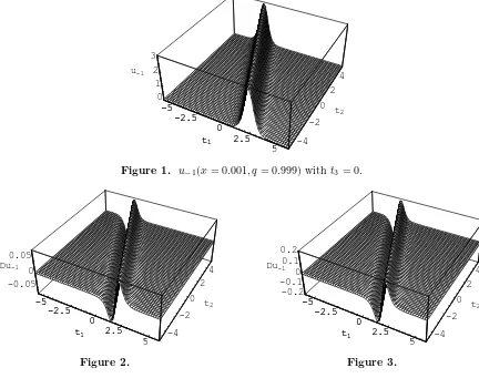
to plot a figure for u−1, we fix λ1 = 2, λ2 = −1.5 and B1 = 1, so u−1 = u−1(x, t1, t2, t3, q).
The single q-soliton u−1(0.001, t1, t2, t3,0.999) is plotted in Fig. 1, which is close to classical
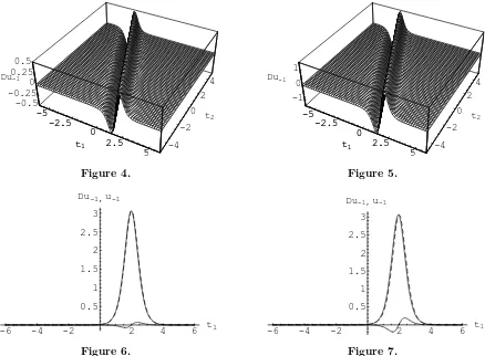
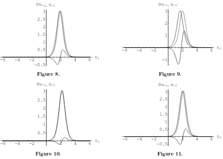
soliton of KP equation as we analysed above. From Figs. 2–52 we can see the varying trends of △u−1 = u−1(0.5, t1, t2,0,0.999)−u−1(0.5, t1, t2,0, q) , u−1(q = 0.999)−u−1(q) for certain
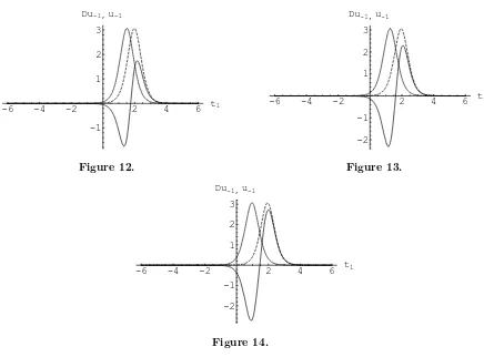
values of q, where q = 0.7,0.5,0.3,0.1 respectively. Furthermore, in order to see the q-effects more clearly, we further fixed t2 = −5 in △u−1, which are plotted in Figs. 6–9. Dependence
of △u−1 = u−1(x, t1,−5,0,0.999)−u−1(x, t1,−5,0,0.1) ,u−1(x, q = 0.999)−u−1(x, q = 0.1)
on x is shown in Figs. 10–14, and x = 0.3,0.4,0.52,0.54,0.55 respectively. It is obvious from figures that △u−1 goes to zero when q →1 and x→0,q-soliton (u−1) of q-KP goes to a usual
soliton of KP, which reproduces the process of q-deformation. On the other hand, Figs. 10–143 show parameterx amplifiesq-effects. In other word, for a given △q,△u−1 will increase along x. However, x is bounded so that eq(λkx) and eq(λkqx) (k = 1,2) are convergent. This is the
reason for plotting u−1 withx≤0.55. Obviously, the convergent interval depends onq and λk.
We would like to emphasize that from Figs. 6–144theq-deformation does not destroy the profile
of soliton; it just similar to an “impulse” to soliton.
5
Symmetry constraint of
q
-KP:
q
-cKP hierarchy
We know that there exists a constrained version of KP hierarchy, i.e. the constrained KP hi-erarchy (cKP) [25, 31], introduced by means of the symmetry constraint from KP hierarchy.
2For Figs. 2–5, q-effect Du
−1 ≡ △u−1 , u−1(q = 0.999)−u−1(q = i) withx = 0.5 and t3 = 0, where i= 0.7,0.5,0.3,0.1. Figs. 6–9, are projection of Figs. 2–5, by fixingt2=−5.
3For Figs. 10–14, the variablex, varies as follows: 0.3,0.4,0.52,0.54,0.55, whileq=i= 0.1 in Du
−1 is fixed. 4For Figs. 6–14, Du
−1,u−1(q= 0.999), are represented by continuous line and dashed line (long), respectively,
-5 -2.5
0 2.5
5
t1 -4
-2 0
2 4
t2 0
1 2 3
u-1
-5 -2.5
0 2.5
[image:17.612.212.414.60.203.2]5 t1
Figure 1. u−1(x= 0.001, q= 0.999) witht3= 0.
-5 -2.5
0 2.5
5
t1 -4
-2 0
2 4
t2 -0.05
0 0.05 Du-1
-5 -2.5
0 2.5
5 t1
Figure 2.
-5 -2.5
0 2.5
5
t1 -4
-2 0
2 4
t2 -0.2
-0.1 0 0.1 0.2
Du-1
-5 -2.5
0 2.5
5 t1
Figure 3.
With inspiration from it, the symmetry of q-KP was established in [22]. In the same article the authors defined one kind of constrainedq-KP (q-cKP) hierarchy by using the linear combination of generators of additional symmetry. In this section, we shall briefly introduce the symmetry and q-cKP hierarchy [22].
The linearization of (2.2) is given by
∂tm(δL) = [δBm, L] + [Bm, δL], (5.1)
where
δBm = m
X
r=1
Lm−rδLLr−1 !
+ .
We call δL=δu0+δu1∂q−1+· · · the symmetry of theq-KP hierarchy, if it satisfies (5.1). LetL
be a “dressed” operator from ∂q, we find
δL=δS∂qS−1−S∂qS−1δSS−1= [δSS−1, L] = [K, L], (5.2)
where δS=δs1∂q−1+δs2∂q−2+· · ·, andK =δSS−1. Therefore
δBm = [K, Lm]+= [K, Bm]+,
the last identity is resulted by K =K− and [K, Lm−]+ = 0. Then the linearized equation (5.1)
is equivalent to
[image:17.612.95.527.65.406.2]-5 -2.5
0 2.5
5
t1 -4
-2 0
2 4
t2 -0.5
-0.25 0 0.25 0.5
Du-1
-5 -2.5
0 2.5
[image:18.612.94.532.57.379.2]5 t1
Figure 4.
-5 -2.5
0 2.5
5
t1 -4
-2 0
2 4
t2 -1
0 1 Du-1
-5 -2.5
0 2.5
5 t1
Figure 5.
-6 -4 -2 2 4 6 t1
0.5 1 1.5 2 2.5 3 Du-1,u-1
Figure 6.
-6 -4 -2 2 4 6 t1
0.5 1 1.5 2 2.5 3 Du-1,u-1
Figure 7.
Let Kn =−(Ln)− (n = 1,2, . . .), then it can easily be checked thatKn satisfies (5.3). For
each Kn,δL is given by δL=−[(Ln)−, L] = [Bn, L] from (5.2). So theq-KP hierarchy admits
a reduction defined by (Ln)−= 0, which is calledq-deformedn-th KdV hierarchy. For example,
n= 2, it leads toq-KdV hierarchy, whose q-Lax operator is
LqKdV =L2=L2+=∂q2+x(q−1)u∂q+u.
There is also another symmetry called additional symmetry, which is K = (MmLl)− [22], and
it also satisfies (5.3). Here the operatorM is defined by
∂tkM = [L +
k, M], M =SΓqS
−1,
and Γq is defined as
Γq =
∞
X
i=1
iti+
(1−q)i
1−qi x i
∂i−1
q .
The more general generators of additional symmetry are in form of
Yq(µ, λ) =
∞
X
m=0
(µ−λ)m m!
∞
X
l=−∞
λ−m−l−1 MmLm+l−,
which are constructed by combination ofK = (MmLl)
−. The operatorYq(µ, λ) can be expressed
as
-6 -4 -2 2 4 6 t1 -0.5
[image:19.612.94.535.53.368.2]0.5 1 1.5 2 2.5 3 Du-1,u-1
Figure 8.
-6 -4 -2 2 4 6 t1
-1 1 2 3 Du-1,u-1
Figure 9.
-6 -4 -2 2 4 6 t1
0.5 1 1.5 2 2.5 3 Du-1,u-1
Figure 10.
-6 -4 -2 2 4 6 t1
-0.5 0.5 1 1.5 2 2.5 3 Du-1,u-1
Figure 11.
In order to define the q-analogue of the constrained KP hierarchy, we need to establish one special generator of symmetryY(t) =φ(t)◦∂−1
q ◦ψ(t) based on Yq(µ, λ), where
φ(t) = Z
ρ(µ)ωq(x, t;µ)dµ, ψ(t) =
Z
χ(λ)θ(ω∗q(x, t;λ))dλ,
furtherφ(t) andψ(t) satisfy (2.12) and (2.13). In other words, we get a new symmetry ofq-KP hierarchy,
K =φ(λ;x, t)◦∂q−1◦ψ(µ;x, t), (5.4)
whereφ(λ;x, t) andψ(µ;x, t) is an “eigenfunction” and an “adjoint eigenfunction”, respectively. We can regard from the process above that K = φ(λ;x, t)◦∂−1
q ◦ψ(µ;x, t) is a special linear
combination of the additional symmetry generator (MmLl)−. It is obvious that generator K
in (5.4) satisfies (5.3), because of the following two operator identities,
(A◦a◦∂q−1◦b)−= (A·a)◦∂q−1◦b,(a◦∂q−1◦b◦A)−=a◦∂q−1◦(A∗·b). (5.5)
Here A is aq-PDO, and aand bare two functions. Naturally, q-KP hierarchy also has a multi-component symmetry, i.e.
K =
n
X
i
φi◦∂q−1◦ψi.
It is well known that the integrable KP hierarchy is compatible with generalizedl-constraints of this type (Ll)
−=P
i
qi◦∂x−1◦ri. Similarly, the l-constraints ofq-KP hierarchy
(Ll)−=K =
m
X
i=1
-6 -4 -2 2 4 6 t1
[image:20.612.93.529.49.371.2]-1 1 2 3 Du-1,u-1
Figure 12.
-6 -4 -2 2 4 6 t1
-2 -1 1 2 3 Du-1,u-1
Figure 13.
-6 -4 -2 2 4 6 t1
-2 -1 1 2 3 Du-1,u-1
Figure 14.
also lead to q-cKP hierarchy. The flow equations of thisq-cKP hierarchy
∂tkL
l= [Lk
+, Ll], Ll= (Ll)++
m
X
i=1
φi◦∂q−1◦ψi (5.6)
are compatible with
(φi)tk = ((L
k)
+φi), (ψi)tk =−((L
∗k)
+ψi).
It can be obtained directly by using the operator identities in (5.5). An important fact is that there exist two m-th orderq-differential operators
A=∂qm+am−1∂qm−1+· · ·+a0, B =∂qm+bm−1∂qm−1+· · ·+b0,
such that ALl and LlB are differential operators. From (ALl)− = 0 and (LlB)− = 0, we get
that A and B annihilate the functions φi and ψi, i.e., A(φ1) = · · · = A(φm) = 0, B∗(ψ1) =
· · ·=B∗(ψ
m) = 0, that impliesφi ∈Ker (A). It should be noted that Ker (A) has dimensionm.
We will use this fact to reduce the number of components of the q-cKP hierarchy in the next section.
6
q
-Wronskian solutions of
q
-cKP hierarchy
We know from Corollary1 thatq-Wronskian
τq(N) =WNq(φ1, . . . , φN) =
φ1 φ2 · · · φN
∂qφ1 ∂qφ2 · · · ∂qφN
..
. ... · · · ...
∂N−1
q φ1 ∂qN−1φ2 · · · ∂qN−1φN
is a τ function of q-KP hierarchy. Here φi (i = 1,2, . . . , N) satisfy linear q-partial differential
equations,
∂φi
∂tn
= (∂qnφi), n= 1,2,3, . . . . (6.2)
In this section, we will reduce τq(N) in (6.1) to a τ function of q-cKP hierarchy. To this end, we
will find the additional conditions satisfied byφi except the linearq-differential equation (6.2).
Corollary 1 also shows that the q-KP hierarchy with Lax operator L(N) =T
N ◦∂q◦TN−1 is
generated from the “free” Lax operatorL=∂q, which has theτ functionτq(N)in (6.1). In order
to get the explicit form of such Lax operator L(N), the following lemma is necessary.
Lemma 5.
TN =
1
WNq(φ1, . . . , φN)
φ1 · · · φN 1
∂qφ1 · · · ∂qφN ∂q
..
. · · · ... ...
∂qNφ1 · · · ∂qNφN ∂qN
and
TN−1 =
φ1◦∂q−1 θ(φ1) · · · θ(∂qN−2φ1) φ2◦∂q−1 θ(φ2) · · · θ(∂qN−2φ2)
..
. ... · · · ...
φN ◦∂q−1 θ(φN) · · · θ(∂qN−2φN)
· (−1)
N−1
θ(WNq(φ1, . . . , φN))
=
N
X
i=1
φi◦∂q−1◦gi
with
gi = (−1)N−iθ
WNq(φ1, . . . , φi−1,ˆi, φi+1, . . . , φN)
WNq(φ1, . . . , φi−1, φi, φi+1, . . . , φN)
. (6.3)
Hereˆi means that the column containingφi is deleted from WNq(φ1, . . . , φi−1, φi, φi+1, . . . , φN),
and the last row is also deleted.
Proof . The proof is a direct consequence of Lemma 3 and Theorem 4 from the initial “free” Lax operator L = ∂q. The generating functions {φi, i = 1,2, . . . , N} of TN satisfies
equa-tions (6.2), which is obtained from definition of “eigenfunction” (2.12) of the KP hierarchy
under Bn=∂qn.
In particular, (TN ·φ1) = (TN ·φ2) =· · ·= (TN·φN) = 0.
Now we can give one theorem reducing the q-Wronskian τ function τq(N) in (6.1) of q-KP
hierarchy to the q-cKP hierarchy defined by (5.6).
Theorem 6. τq(N) is also a τ function of theq-cKP hierarchy whose Lax operatorLl= (Ll)++
M
P
i=1
qi◦∂q−1◦ri with some suitable functions{qi, i= 1,2, . . . , M}and{ri, i= 1,2, . . . , M}if and
only if
WNq+M+1(φ1, . . . , φN, ∂qlφi1, . . . , ∂
l
qφiM+1) = 0 (6.4)
for any choice of (M + 1)-indices (i1, i2, . . . , iM+1) 1 6 i1 < · · · < iM+1 ≤ N, which can be expressed equivalently as
WMq+1 W
q
N+1(φ1, . . . , φN, ∂qlφi1) WNq(φ1, . . . , φN)
,W
q
N+1(φ1, . . . , φN, ∂qlφi2) WNq(φ1, . . . , φN)
WNq+1(φ1, . . . , φN, ∂qlφiM+1) WNq(φ1, . . . , φN)
!
= 0 (6.5)
for all indices. Here {φi, i= 1,2, . . . , N} satisfy (6.2).
Remark 4. This theorem is a q-analogue of the classical theorem on cKP hierarchy given by [38].
Proof . The q-Wronskian identity proven in Appendix C
WMq+1 W
q
N+1(φ1, . . . , φN, f1) WNq(φ1, . . . , φN)
, . . . ,W
q
N+1(φ1, . . . , φN, fM+1) WNq(φ1, . . . , φN)
!
= W
q
N+M+1(φ1, . . . , φN, f1, . . . , fM+1) WNq(φ1, . . . , φN)
implies equivalence between (6.4) and (6.5). Using TN and TN−1 in Lemma 5 and the operator
identity in (5.5) we have
(Ll)−= (TN ◦∂ql ◦TN−1)−=
N
X
i=1
(TN(∂qlφi))◦∂−q1◦gi, (6.6)
where gi is given by (6.3) and TN acting on (∂qlφi) is TN(∂qlφi) =
WNq+1(φ1, φ2, . . . , φN, ∂qlφi)
WNq(φ1, φ2, . . . , φN)
.
So τq(N) is automatically a tau function ofN-component q-cKP hierarchy with the form (6.6).
Next, we can reduce theN-component to the M-component (M < N) by a suitable constraint of φi.
Suppose that theM-component (M < N)q-cKP hierarchy is obtained by constraint of qKP hierarchy generated by TN, i.e., there exist suitable functions{qi, ri} such that
(Ll)−=
M
X
i=1
qi◦∂q−1◦ri= N
X
i=1
(TN(∂qlφi))◦∂q−1◦gi.
As we pointed out in previous section, for a Lax operator whose negative part is in the form of
(Ll)
− =
M
P
i=1
qi◦∂q−1◦ri, there exists an M-th order q-differential operator A such that ALl is
a q-differential operator, then we have
0 =ALl(TN(φi)) =ATN∂ql(φi) =A(TN(∂qlφi))
from TN(φi) = 0that implies TN(∂qlφi) ∈ Ker (A). Therefore, at most M of these functions
TN(∂qlφi) can be linearly independent because the Kernel of A has dimension M. So (6.5) is
deduced.
Conversely, suppose (6.5) is true, we will show that there exists one M-component q-ckP (M < N) constrained from (6.6). The equation (6.5) implies that at most M of functions TN(∂qlφi) (i = 1,2, . . . , N) are linearly independent. Then we can find suitable M functions {q1, q2, . . . , qM}, which are linearly independent, to express functionsTN(∂qlφi) as
TN(∂qlφi) =
WNq+1(φ1, φ2· · · , φN, ∂qlφi)
WNq(φ1, φ2, . . . , φN)
=
M
X
j=1
with some constants cij. Taking this back into (6.6), it becomes
(Ll)−=
N
X
i=1
M
X
j=1 cijqj
◦∂−q1◦gi= M
X
j=1
qj◦∂q−1◦ N
X
i=1 cijgi
! =
M
X
j=1
qj◦∂q−1◦rj,
which is anM-componentq-cKP hierarchy as we expected.
7
Example reducing
q
-KP to
q
-cKP hierarchy
To illustrate the method in Theorem6reducing theq-KP to multi-component aq-cKP hierarchy, we discuss the q-KP generated by TN|N=2. In order to obtain the concrete solution, we only
consider the three variables (t1, t2, t3) in t. Furthermore, the q1,r1 and u−1 are constructed in
this section.
According to Theorem6, theq-KP hierarchy generated byTN|N=2 possesses a tau function
τq(2) =W2q(φ1, φ2) =φ1(∂qφ2)−φ2(∂qφ1)
= (λ2−λ1)eq(λ1x)eq(λ2x)eξ1+ξ2 + (λ3−λ1)eq(λ1x)eq(λ3x)eξ1+ξ3
+ (λ3−µ)eq(µx)eq(λ3x)eξ+ξ3 + (λ2−µ)eq(µx)eq(λ2x)eξ+ξ2 (7.1)
with
φ1 =eq(λ1x)eξ1 +eq(µx)eξ, φ2=eq(λ2x)eξ2 +eq(λ3x)eξ3.
Hereξi =ci+λit1+λ2it2+λ3it3 (i= 1,2,3), andξ=d+µt1+µ2t2+µ3t3,ciand dare arbitrary
constants. These functions satisfy the linear equations
∂φi
∂tn
=∂qnφi, n= 1,2,3, i= 1,2,
as a special case of (6.2). From (6.6), theq-KP hierarchy generated byTN|N=2 is in the form of
Ll = (Ll)++ (T2(∂qlφ1))◦∂q−1◦g1+ (T2(∂qlφ2))◦∂−q1◦g2, (7.2) constraint
===== (Ll)++q1◦∂q◦r1. (7.3)
Here q1 and r1 are undetermined, which can be expressed byφ1 andφ2 as follows.
According to (6.4), the restriction forφ1 and φ2 to reduce (7.2) to (7.3) is given by
0 =W2q(φ1, φ2, ∂qlφ1, ∂qlφ2) = (µl−λl1)(λl2−λl3)V(λ1, λ2, λ3, µ)ec1+c2+c3+de(λ1+λ2+λ3+µ)t1
×e(λ21+λ22+λ23+µ2)t2e(λ31+λ32+λ33+µ3)t3e
q(λ1x)eq(λ2x)eq(λ3x)eq(µx) (7.4)
with
V(λ1, λ2, λ3, µ) =
1 λ1 λ21 λ31
1 λ2 λ22 λ32
1 λ3 λ23 λ33
1 µ µ2 µ3 .
Obviously, we can letµ=λ2andd=c2such that (7.4) holds forφ1andφ2. Then theτ function
of a single component q-cKP defined by (7.3) is
+ (λ3−λ2)eq(λ2x)eq(λ3x)eξ2+ξ3,
which is deduced from (7.1). That means we indeed reduce the τ function τq(2) in (7.1) of
the q-KP hierarchy generated by TN|N=2 to the τ functionτqcKP of the one-component q-cKP
hierarchy. Furthermore, we would like to get the explicit expression of (q1, r1) of q-cKP in (7.3).
Using the determinant representation ofTN|N=2 and TN−1|N=2, we have
f1 ,(T2(∂qlφ1)) =
(λl1−λl2)(λ3−λ2)(λ2−λ1)(λ3−λ1)eq(λ1x)eq(λ2x)eq(λ3x)eξ1+ξ2+ξ3 τqcKP
,
f2 ,(T2(∂qlφ2) =
(λl
3−λl2)(λ3−λ2)(λ2−λ1)(λ3−λ1)eq(λ1x)eq(λ2x)eq(λ3x)eξ1+ξ2+ξ3 τqcKP
,
g1 =−θ
φ2 τqcKP
, g2=θ
φ1 τqcKP
,
under the restriction µ= λ2 and d=c2. One can find that f1 and f2 are linearly dependent,
and (λl3−λl2)f1 = (λl1−λl2)f2. So (7.2) and (7.3) reduce to
Ll−=f1◦∂q−1◦g1+f2◦∂q−1◦g2
= (λl3−λl2)f1◦∂q−1◦
g1
(λl3−λl2) + (λ
l
1−λl2)f2◦∂q−1◦
g2
(λl1−λl2) =q1◦∂
−1
q ◦r1,
in which
q1 ,(λl3−λl2)f1 = (λl1−λl2)f2
= (λ
l
1−λl2)λl3−λl2)(λ3−λ2)(λ2−λ1)(λ3−λ1)eq(λ1x)eq(λ2x)eq(λ3x)eξ1+ξ2+ξ3 τqcKP
,
r1,
g1
(λl
3−λl2)
+ g2
(λl
1−λl2)
= 1
(λl
1−λl2)(λl3−λl2)
×θ e
−(ξ1+ξ2+ξ3) (λl
3−λl2)eq(λ1x)eξ1 + (λl3−λl1)eq(λ2x)eξ2 + (λl2−λl1)eq(λ3x)eξ3 τqcKP
! .
In particular, we can let λ1 =λ,λ2 = 0,λ3=−λ,c1 =c,c2 =−0,c3 =−c,then
q1 =
(−1)lλ2l+2eq(λx)eq(−λx)
eq(λx)eq(−λx) +eq(λx)e
η+e
q(−λx)e−η
2 e−λ
2t2
and
r1=
− 1
λl+1θ "
e−λ2t
2+eq(λx)eη+eq(−λx)e−η 2
eλ2t2
eq(λx)eq(−λx) +eq(λx)e
η+e
q(−λx)e−η 2
#
ifl is odd,
− 1
λl+1θ
" eq(λx)eη−e
q(−λx)e−η 2
eλ2t2
eq(λx)eq(−λx) +eq(λx)e
η+e
q(−λx)e−η 2
#
ifl is even,
where η=c+λt1+λ3t3.
In general, thel-constrained one-component q-KP hierarchy has the Lax operatorL=∂q+
u0+q1 ◦∂q−1◦r1 when l = 1. On the other hand, its Lax operator can also be expressed as L=∂q+u0+u−1∂q−1+u−2∂−q2+· · ·. So all of the dynamical variables {u−i, i= 1,2,3, . . .}of
q-KP hierarchy are given by
-10 -5
0
5
10 t1
-2 -1
0 1
2 3
t2 0
1 2 3 u-1
-10 -5
0
[image:25.612.213.413.58.206.2]5 t1
Figure 15. u−1(x= 0.001, q= 0.999) fromq-cKP and t3= 0.
For the present situation, u−1 = u−1(t1, t2, t3) = q1θ−1(r1) represents the q-deformed solution
of the classical KP eqution, which is constructed from the components of q-cKP hierarchy, and is of the form
q1 =
−λ4eq(λx)eq(−λx)
eq(λx)eq(−λx) +eq(λx)e
η+e
q(−λx)e−η
2 e−λ
2t2, (7.5)
r1=− 1 λ2θ
"
e−λ2t
2+ eq(λx)eη+eq(−λx)e−η 2
eλ2t2
eq(λx)eq(−λx) +eq(λx)e
η+e
q(−λx)e−η 2
#
, (7.6)
u−1 =
λ2eq(λx)eq(−λx)
eq(λx)eq(−λx) +eq(λx)e
η+e
q(−λx)e−η
2 e−λ
2t2
× e
−λ2t
2+ eq(λx)eη+eq(−λx)e−η 2
eλ2t2
eq(λx)eq(−λx) +eq(λx)e
η+e
q(−λx)e−η
2
. (7.7)
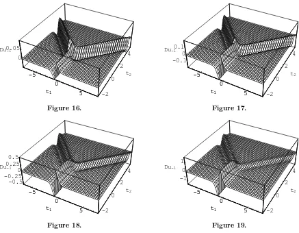
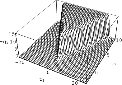
Obviously, they will approach to the classical results on the cKP hierarchy in [38] when x → 0 and q → 1. We will fix λ = 2, t3 = 0 and c = 0 to plot their figures, then get q1=q1(x, t1, t2, q),r1 =r1(x, t1, t2, q) andu−1 =u−1(x, t1, t2, q) from (7.5)–(7.7). To save space,
we plot the figures foru−1 and q1 in (t1, t2, t3) dimension spaces. It can be seen that Fig. 15 of u−1(0.001, t1, t2,0.999) and Fig. 20 of q1(0.001, t1, t2,0.999) match with the profile ofu1 and q
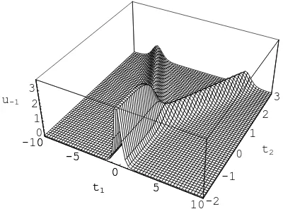
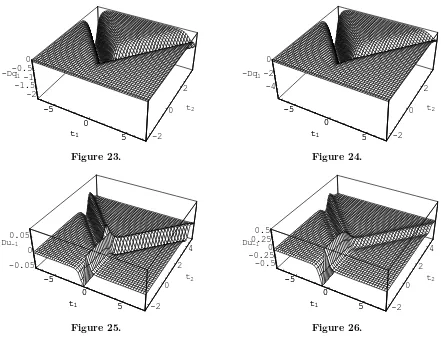
in [38] with the same parameters. So we defineq-effects quantity△u−1 =u−1(0.5, t1, t2,0.999)− u−1(0.5, t1, t2, q) =u−1(q = 0.999)−u−1(q),△q1=q1(0.5, t1, t2,0.999)−q1(.5, , t1, t2, q) =q1(q =
0.999)−q1(q), to show their dependence on q. Figs. 16–195 and Figs. 21–246 are plotted for
△u−1 and △q1, respectively, where q = 0.7,0.5,0.3,0.1. Obviously, they are decreasing to
almost zero when q goes from 0.1 to 1 with fixedx= 0.5. Furthermore, Figs. 25–297 show that
the dependence of the q-effects △u−1 = u−1(x, t1, t2,0.999)−u−1(x, t1, t2,0.1) = u−1(x, q =
0.999)−u−1(x, q = 0.1) on x,where x = 0.2,0.4,0.51,0.53,0.55 in order. These figures give
us again an opportunity to observe the process of q-deformation in q-soliton solution of q-KP equation. They also demonstrate that q-deformation keep the profile of the soliton, although there exists deformation in some degree. On the other hand, in fact, (q1, r1) can be regarded as
5For Figs. 16–19, q-effect Du
−1 ≡ △u−1 , u−1(q = 0.999)−u−1(q = i), wherei = 0.7,0.5,0.3,0.1, from q-cKP withx= 0.5 andt3= 0.
6For Figs. 21–24,q-effect Dq
1≡ △q1,q1(q= 0.999)−q1(q=i), wherei= 0.7,0.5,0.3,0.1, fromq-cKP with x= 0.5 andt3= 0.
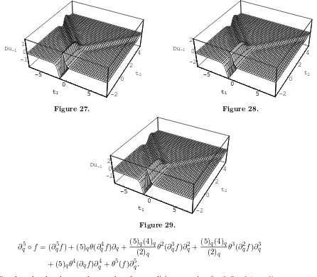
7For Figs. 25–29,
q-effect Du−1≡ △u−1,u−1(x=i, q= 0.999)−u−1(x=i, q= 0.1) fromq-cKP witht3= 0,
-5
0
5
t1 -2
0 2
4
t2 0
0.05 Du-1
-5
0
[image:26.612.95.532.54.394.2]5 t1
Figure 16.
-5
0
5
t1 -2
0 2
4
t2 -0.1
0 0.1 Du-1
-5
0
5 t1
Figure 17.
-5
0
5
t1 -2
0 2
4
t2 -0.5
-0.25 0 0.25 0.5
Du-1
-5
0
5 t1
Figure 18.
-5
0
5
t1 -2
0 2
4
t2 -1
0 1 Du-1
-5
0
5 t1
Figure 19.
a q-deformation of dynamical variables (q, r) of AKNS hierarchy, because cKP possessing Lax operatorL=∂+q◦∂−1◦r is equivalent to the AKNS hierarchy.
8
Conclusions and discussions
In this paper, we have shown in Theorem 1 that there exist two types of elementary gauge transformation operators for the q-KP hierarchy. The changing rules ofq-KP under the gauge transformation are given in Theorems2 and3. We mention that these two types of elementary gauge transformation operators are introduced first by Tu et al. [15] for q-NKdV hierarchy. Considering successive application of gauge transformation, we established the determinant rep-resentation of the gauge transformation operator of the q-KP hierarchy in Lemma 3 and the corresponding results on the transformed new q-KP are given in Theorem 5. For the q-KP hierarchy generated by Tn+k from the “free” Lax operator L = ∂q (i.e. the Lax operator is
L(n+k)=Tn+k◦∂q◦Tn−+1k), Corollary 1shows that the generalized q-WronskianIWk,nq of
func-tions{φi, ψj}(i= 1,2, . . . , n;j= 1,2, . . . , k) is a generalτ function of it, andq-WronskianWnq
of functions φi(i = 1,2, . . . , n) is also a special one. Here {φi} and {ψj} satisfy special linear
q-partial differential equations (4.5).
The symmetry and symmetry constraint ofq-KP (q-cKP) hierarchy are discussed in Section 5. On the basis of the representation of TN in Lemma 5, the q-KP hierarchy whose Lax operator
Ll =TN ◦∂lq◦TN−1 is generated from the “free” Lax operator L=∂q. The explicit form of its
-20
0
20 t1
0 5
10
t2 0
5 10 15
-q1
-20
0
[image:27.612.215.411.59.195.2]20 t1
Figure 20. q1(x= 0.001, q= 0.999) andt3= 0.
-5
0
5
t1 -2
0 2
t2 -0.4
-0.3 -0.2 -0.1 0
-Dq1
-5
0
[image:27.612.96.530.226.394.2]