Electronic Journal of Qualitative Theory of Differential Equations
2010, No. 60, 1-32;http://www.math.u-szeged.hu/ejqtde/
FRACTAL ANALYSIS OF HOPF BIFURCATION FOR A CLASS OF
COMPLETELY INTEGRABLE NONLINEAR SCHR ¨ODINGER CAUCHY
PROBLEMS
JOSIPA PINA MILIˇSI ´C, DARKO ˇZUBRINI ´C, AND VESNA ˇZUPANOVI ´C
Abstract. We study the complexity of solutions for a class of completely integrable, nonlinear integro-differential Schr¨odinger initial-boundary value problems on a bounded domain, depending on a real bifurcation parameter. The considered Schr¨odinger prob-lem is a natural extension of the classical Hopf bifurcation model for planar systems into an infinite-dimensional phase space. Namely, the change in the sign of the bifurcation parameter has a consequence that an attracting (or repelling) invariant subset of the sphere in L2(Ω) is born. We measure the complexity of trajectories near the origin by
considering the Minkowski content and the box dimension of their finite-dimensional pro-jections. Moreover we consider the compactness and rectifiability of trajectories, and box dimension of multiple spirals and spiral chirps. Finally, we are able to obtain the box di-mension of trajectories of some nonintegrable Schr¨odinger evolution problems using their reformulation in terms of the corresponding (not explicitly solvable) dynamical systems inRn
.
Corresponding author: Josipa Pina Miliˇsi´c
University of Zagreb, Faculty of Electrical Engineering and Computing Unska 3, 10000 Zagreb, Croatia
1. Introduction
1.1. Motivation and formulation of the problem. Dimension theory for dynamical systems has been rapidly developed due to its important applications in other natural, social and technical sciences. Since the early 1970’s scientists have started to estimate and compute fractal dimensions of strange attractors for finite (Lorenz, Henon, Chua, Leonov, etc.), as well as for the infinite-dimensional dynamical systems (Ladyzhenskaya, Foia¸s and Temam, Babin and Vishik, Ruelle, Lieb, etc.) Fractal dimensions in dynamics are discussed in a survey article [29]. However, our approach to the question of fractal dimensions in dynamics is different in a way that we are interested in the complexity of trajectories of dynamical systems and study the dependence of the computed fractal dimension upon the bifurcation parameter. Knowing the information about fractal dimension of trajectories
1991Mathematics Subject Classification. 35Q55, 37G35, 28A12, 34C15.
Key words and phrases. Schr¨odinger equation, Hopf bifurcation, box dimension, Minkowski content, compactness, rectifiability, bundle of trajectories, oscillation, multiple spiral, spiral chirp.
enables to measure the complexity of the studied dynamics which we mostly describe by calculating the corresponding box dimension and, in order to describe finer properties, its Minkowski content. Namely, the Hausdorff dimension of trajectories that we are interested in, is always trivial.
The second and third author have undertaken a systematic study of fractal properties of trajectories of vector fields near the weak focus inR2 and analogously inR3. Furthermore,
they considered a connection between the box dimension of the trajectory and the bifur-cation of the related dynamical system. Here we mention that this interesting connection has been studied also in [10, 16] but for one-dimensional discrete dynamical systems.
In this article, using methods developed in [20, 26, 27, 28] we consider the trajectories of vector fields in infinite-dimensional case and we calculate their box dimensions. The original idea of this paper grounds on the connection between nonlocal Schr¨odinger evo-lution problems and the corresponding system of ODE’s. More precisely, starting from completely integrable nonlinear integro-differential Schr¨odinger equation we arrive at an equivalent system of infinitely many nonlinear ODE’s. Concerning the observed link be-tween Schr¨odinger problems and vector fields it is interesting to point out that each pla-nar system of ODE’s with polynomial right-hand side can be interpreted as a nonlinear Schroedinger equation with an explicit corresponding nonlinear term. Moreover, as it is described in Section 6.3, this consideration is valid even for any dynamical system in Rn.
Therefore, it is worth noting that the 16th Hilbert problem about the search of an uniform upper bound for the number of limit cycles in polynomial vector fields can be considered in terms of a Schr¨odinger equation.
In ˇZubrini´c and ˇZupanovi´c [26, Theorem 9] it has been shown that the box dimension of spiral trajectories of the classical Hopf bifurcation system in the plane described by (4), viewed near the focus, is equal to d = 4/3 when the bifurcation parameter a0 is equal
0. Furthermore, these trajectories are Minkowski nondegenerate, i.e. their d-dimensional Minkowski contents, are different from 0 and ∞. On the other hand, for a0 6= 0 all
We start with the Cauchy problem for the following nonlinear Schr¨odinger (NLS) initial-boundary value problem:
(1)
ut(t, x) = i∆u(t, x)−γ u(t, x)
Z
Ω|
u(t, x)|2dx+a0
u(t, x) = 0 for x∈∂Ω, t∈(tmin, tmax)
u(0, x) = u0(x) for x∈Ω.
where i is the imaginary unit, γ is a fixed nonzero complex number, a0 a real bifurcation
parameter, Ω a bounded domain inRN, N ≥1, andu0 : Ω→Cis a given initial function,
u0 ∈L2(Ω,C). Here ∆u=PNj=1 ∂
2
u ∂x2
j is the Laplace operator. For a fixed space variable x, the solutionsu: (tmin, tmax)→L2(Ω,C) of the NLS Cauchy problem (1) can be considered
as trajectories in the Hilbert space L2(Ω,C) where L2(Ω,C) = L2(Ω) +iL2(Ω) is the
complexification of the real spaceL2(Ω). We point out thatt
min and tmax depend on γ,a0
and u0, and 0∈(tmin, tmax). In this article, we are dealing with unbounded time intervals
(tmin, tmax) either of the form (tmin,∞), or (−∞,∞), or (−∞, tmax).
Due to the integral term in (1), this NLS Cauchy problem is of nonlocal type. Similar nonlocal problems with the same integral term have been considered for the modified cubic wave equation,
utt−∆u+c
Z
Ω
u(t, x)2dx
u= 0,
with homogeneous Dirichlet boundary condition, in Cazenave, Haraux and Weissler [3, 4, 5], in their study of completely integrable abstract wave equations. We consider the Schr¨odinger equation (1) fora0 = 0 as an approximation of the equationut =i∆u−γu|u|2
following the approach of [5, p. 130].
The same integral term as in (1) can be seen in Christ [8, pp. 132 and 133]. An analogous one appears in an equation of fourth order arising from the theory of aeroelasticity,
uxxxx+
α−β
Z 1
0
u2xdx
uxx+γux+δut+εutt = 0
see Chicone [7, p. 310]. Other integro-differential Schr¨odinger problems involving different integral operators on the right-hand side have been studied in numerous papers, see for example Chen and Guo [6].
1.2. Interpretation in ℓ2. In order to write down problem (1) as an infinite system of
nonlinear ordinary differential equations we exploit a well known Fourier series expansion using the decomposition with respect to a Hilbert basis in L2(Ω). Let (ϕ
j) be the
or-thonormal basis of eigenfunctions of the operator −∆ with zero boundary data and with eigenvalues (λj) such that 0 < λ1 < λ2 ≤ λ3 ≤ . . . (see e.g. Brezis [1, ersatz (12) on p.
an orthonormal base in L2(Ω,C). By writing the solution u(t, x) in the form:
(2) u(t, x) =
∞ X
j=1
zj(t)ϕj(x),
the NLS Cauchy problem (1) formally reduces to a lattice Schr¨odinger equation on the Hilbert space of quadratically summable sequences of complex numbers, which we denote by ℓ2(C). More precisely, we obtain an infinite system of nonlinear ODE’s:
(3) z˙j =−iλjzj−γzj(kzk2+a0), j = 1,2, . . . ,
with initial condition zj(0) = zj0, j ≥ 1, where (zj0) ∈ ℓ2(C) and z(t) = (zj(t))j ∈ ℓ2(C)
for each t ∈(tmin, tmax). Clearly, zj0 =hu0, ϕji=
R
Ωu0ϕjdx and k · k is a standard Euclid
norm. For given u0 ∈L2(Ω,C), we interpret NLS equation (1)1 as the lattice Schr¨odinger
equation (3). To any v ∈L2(Ω,C) one can assign z = (z
j)j ∈ℓ2(C), where v =Pjzjϕj is
the Fourier expansion of v, and this assignment is an isometric isomorphism.
Here, we note that the NLS Cauchy problem (1) is a natural extension of the Hopf bifurcation model for planar systems. The Hopf bifurcation is connected to 1-parameter families of vector fields where a limit cycle surrounding a singular point is born. It is well known that the Hopf bifurcation occurs at an equilibrium point x0 of a planar system
˙
x= f(x, a0) depending on a parameter a0 ∈ R when the matrix Df(x0, a0) has a pair of
pure imaginary eigenvalues, see [21, pg. 314.]. In this sense we say that the pointx0 is the
weak focus of the system. On the other side, if the eigenvalues are such that both their real and imaginary parts differ from zero, we are speaking about the strong focus.
Namely, when z = (z1,0,0, . . .), and assuming that λ1 = 1, γ = 1, the system (3)
reduces to the classical Hopf bifurcation system in the plane:
(4)
˙
x = y−x(x2 +y2+a 0)
˙
y = −x−y(x2+y2+a 0),
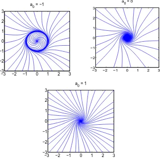
where we denote x(t) = Rez(t), y(t) = Imz(t), real and imaginary part of the complex number z(t), respectively. System (4) written using the polar coordinates (r, θ) reads
˙
r=r(r2+a0), θ˙=−1.
(5)
and can be explicitly solved. Since ˙θ 6= 0, the originr= 0 is the only critical point. Since ˙
θ <0 the flow is always clockwise. The phase portrait of (4) fora0 <0,a0 = 0 and a0 >0
is shown by Figure 1. Viewing a0 as the bifurcation parameter, we point out the following
cases in which the stability of the origin changes, i.e. the bifurcation occurs:
(i) For a0 > 0 the origin is unstable strong focus and for all trajectories we have
(tmin, tmax) = (−∞, t0) with tmax =t0 >0.
(ii) Fora0 = 0 the origin is unstable weak focus, and (tmin, tmax) = (−∞, t0), t0 >0.
(iii) For a0 < 0 the origin is a stable strong focus. The limit cycle is the circle of
−3 −2 −1 0 1 2 3 −3
−2 −1 0 1 2 3
a
0 = −1
−3 −2 −1 0 1 2 3
−3 −2 −1 0 1 2 3
a 0 = 0
−3 −2 −1 0 1 2 3
−3 −2 −1 0 1 2 3
a
[image:5.595.147.469.98.422.2]0 = 1
Figure 1. Phase portrait of the classical Hopf bifurcation system (4).
are global, i.e. (tmin, tmax) = (−∞,∞), while for those outside the circle we have
(tmin, tmax) = (t0,∞) with t0 <0.
Next, let us consider the Hopf bifurcation in a complex system (3), but in finite-dimensional phase space. We start with two-finite-dimensional complex system
(6) z˙j =−iλjzj −γzj(|z1|2+|z2|2+a0), j = 1,2,
with the corresponding initial conditionszj(0) =zj0, wherea0 is the bifurcation parameter.
To simplify, for the moment we assume that γ ∈ R and γ >0. Near a0 = 0 we have the
qualitative change of the behavior of the system. Indeed, using the polar coordinates the system (6) can be written as
˙
where zj =rjexp(iθj). For a0 <0 an invariant set, 3-sphere
√
−a0S3 ={(z1, z2)∈R4: |z1|2+|z2|2 =−a0,}
(7)
in R4 is born, where S3 is the unit sphere in R4. In analogy with the case of R2, we call
this phenomenon the Hopf bifurcation in R4. Clearly, if a
0 →0−, then the sphere shrinks
to the origin. Moreover, if r2
1 +r22 <−a0, then ˙rj < 0, and r(t) is decreasing as t → ∞. The α-limit
set of the trajectory is the origin, while the ω-limit set is a subset of the sphere (7). More precisely, the corresponding limit set is the subset of the 2-torus, contained in the 3-sphere (7). The torus has the form
r1S1×r2S1 ⊂√−a0S3,
wherer1,2are positive scaling numbers depending on the initial point,r12+r22 =−a0, andS1
is the unit circle in the complex planeC. Clearly, ifr2
1+r22 >−a0, andr(t) monotonically
increases, then the corresponding trajectories converge to the sphere and their ω-limit set is a subset of a 2-torus contained in the 3-sphere (7).
In the similar way the Hopf bifurcation for the following system ofk complex equations: (8) z˙j =−iλjzj −γzj(|z1|2+· · ·+|zk|2+a0), j = 1,2, . . . , k,
can be understood. An invariant (2k−1)-sphere is born in Ck when a0 < 0, defined by |z1|2+· · ·+|zk|2 =−a0. For the general theory of bifurcation problems in finite-dimensional
dynamical systems see Guckenheimer and Holmes [13].
1.3. Hopf bifurcation in an infinite-dimensional phase space. Since we are inter-ested in the phenomenon of the Hopf bifurcation in an infinite-dimensional complex system (3), we start with the description of the Hopf bifurcation for an ODE defined in a Banach space X (real or complex):
(9) u˙ =F(u, a0), u(0) =u0.
Here F : D×R → X is a given map, where D is a dense subspace of X, and the initial
valueu0 ∈D is prescribed. For our purposes the mapping F is usually of the form
F(u, a0) =Au+f(u, a0),
where A:D⊆X →X is a second order differential operator,f: X×R→X continuous
such that f(u,0) = o(u) as u → 0, and a0 is the bifurcation parameter. Additionally we
assume that for alla0 we haveF(0, a0) = 0 so thatu= 0 is an equilibrium point. For each
initial point u0 in a neighbourhood of 0∈D let a trajectory
Γ(u0) ={u(t)∈X: t∈(tmin, tmax), u(0) =u0}
(10)
of (9) be defined on an unbounded interval (tmin, tmax) containing the origin.
Definition 1. We say thata0 = 0 is the point ofHopf bifurcationfor the system (9) if the
(i) Fora0 ≥0 small enough the system is unstable near the origin, and for u0 from a
neighbourhood of the origin we have (tmin, tmax) = (−∞, t0),tmax=t0 >0.
(ii) For a0 < 0 with |a0| small enough, the origin is stable, and an unstable invariant
set S(a0)⊂X for (9) is born near the origin. There exists an open neighbourhood
U(a0) of the origin such that its boundary is S(a0), and for any u0 ∈ U(a0) the
corresponding solution is global, i.e. (tmin, tmax) = (−∞,∞), while for u0 ∈ B \
U(a0) we have that (tmin, tmax) = (−∞, t0) with t0 >0.
Definition 1 is analogous if the signs ofa0 are reversed, in which case the stability should
be reversed as well as semi-infinite time intervals. Somewhat loosely we say that the Hopf bifurcation occurs if an invariant set is born near the origin when a0 passes through the
value of 0, and the origin changes from stable to unstable or vice versa.
Returning to the NLS Cauchy problem (1), the Hopf bifurcation consists in thebirth of an invariant sphere in the space L2(Ω) when a
0 < 0. Here we introduce some notation.
Fora0 <0 we define R=√−a0 and let
BR(0) ={v ∈L2(Ω) : kvkL2(Ω) < R}, SR(0) =∂BR(0), (11)
be the ball and the sphere in L2(Ω), respectively. In the same way, when a
0 < 0 for
the corresponding system (3) in ℓ2(C), the Hopf bifurcation consists in the birth of an
invariant sphere in the space ℓ2(C). Since (8) is also a special case of the NLS Cauchy
problem (1), corresponding to the case when u0 ∈ span{ϕ1, . . . , ϕk}, we see that we can
expect trajectories of (1) in the Hilbert space L2(Ω,C), which oscillate at infinitely many
scales. We can achieve this by choosing u0 so that hu0, ϕji 6= 0 for infinitely manyj’s.
Furthermore, we are interested in Hopf bifurcations from the point of view of fractal geometry. For that purpose, in the next subsection firstly we review some standard notation and definitions from fractal geometry and Sobolev spaces.
1.4. Notation and definitions. Let A be a bounded set in Rk, and let d(x, A) be
Eu-clidean distance fromxtoA. Then theMinkowski sausageAεisAε:={y∈Rkd(y, A)< ε},
a term coined by B. Mandelbrot. By lower s-dimensional Minkowski content of A, s ≥0, we mean the following:
(12) Ms∗(A) := lim inf
ε→0
|Aε|
εk−s,
where | · | is N-dimensional Lebesgue measure. Analogously for the upper s-dimensional Minkowski content of A. The lower box dimension ofA is defined by
dimBA= inf{s >0 :Ms∗(A) = 0},
and analogously the upper box dimension dimBA. For various properties of fractal
If A is such that dimBA = dimBA, then the common value is denoted by d:= dimBA,
and is called the box dimension of A. Furthermore, if both the upper and lower d -dimensional Minkowski contents of Aare different from 0 and ∞, we say that the set A is Minkowski nondegenerate. If in addition to this we have Md
∗(A) = M∗d(A) =: Md(A) ∈ (0,∞), then A is said to be Minkowski measurable. The notion of Minkowski content appears for example in the study of fractal drums and fractal strings, see He and Lapidus [14], Lapidus and Frankenhuysen [18]. Furthermore, Minkowski content is essential for understanding some singular integrals, see [25].
If A is a subset of an infinite-dimensional vector space X, we say that dimBA = ∞
if there exists an increasing sequence of finite-dimensional subspaces Xk of X such that
dimB(A∩Xk)→ ∞ ask → ∞. We need this definition in Theorem 6(b).
We deal with the Sobolev spaces H1
0(Ω,C) and H01(Ω,C)∩H2(Ω,C) (in the sequel we
omit C) equipped with the corresponding norms defined by
(13) ku0k2H1 0 =
X
j
λj|hu0, ϕji|2, ku0k2H1 0∩H
2 = X
j
λ2j|hu0, ϕji|2.
See Henry [1, 15].
All the results of this paper hold if in (1) we have−∆ instead of ∆. Thej-th component of trajectory, viewed as a spiral inC, only changes the orientation for eachj from negative
to positive, see (18) below.
2. Well-posedness and stability of solutions
2.1. Explicit solutions of the NLS problem. We consider the NLS initial-boundary value problem (1). For some special values of parameters γ and a0 it is possible to find
explicit solutions of problem (1) and then to consider their qualitative properties. In order to calculate directly the explicit solutions of problem (1), we need the following lemma.
Lemma 2. Let u be a solution of the NLS Cauchy problem (1) in the form (2). Further-more, let ρ(t) =ku(t)kL2, zj(t) =rj(t) exp(iθj(t)), and V(ρ) =ρ2+a0. Then
˙
ρ=−γ1ρV(ρ)
˙
rj =−γ1rjV(ρ), j ∈N
(14)
˙
θj =−λj−γ2V(ρ), j ∈N,
where γ =γ1 +iγ2. Furthermore, for u0 6= 0 we have
(15) rj(t) = |h
u0, ϕji|
ku0kL2
ρ(t).
Proof. In Section 1, we showed that the NLS Cauchy problem (1) can be written in the form on an infinite-dimensional ODE system
˙
zj =−iλjzj −γV(ρ)zj, j ∈N,
where zj = rjexp(iθj). The expressions (14)2 and (14)3 follow easily by multiplying the
expression (16) by exp(−iθj). The first equation in (14) we get directly from the formal
calculation. Namely,
2ρρ˙ = d dt
Z
Ω|
u(t)|2dx=
Z
Ω
d
dt(u(t)u(t))dx=
Z
Ω
( ˙u(t)u(t) +u(t) ˙u(t))dx
= i
Z
Ω
(∆u(t)u(t)−u(t) ∆u(t))dx−2γ1
Z
Ω|
u(t)|2dx·V(ku(t)kL2)
= −2γ1ρ2V(ρ).
By dividing the first two expressions given in (14) we obtain ˙
rj
rj
= ρ˙ ρ,
hence rj = Cjρ, where Cj is a constant depending on the initial value u0. Using the
expression (2), we obtain that
cj = |h
u0, ϕji|
ku0kL2
e−iθj(0),
where hu0, ϕji=
R
Ωu0ϕjdx∈C.
Next, we use the results given by lemma 2 in order to find the explicit solutions of the NLS Cauchy problem (1) for some special values of the parameters γ and a0. We use the
notationρ0 =ku0kL2. For the sake of simplicity we takeγ2 = 0, i.e. γ ∈R. Case 1: a0 ∈R,γ1 = 0.
¿From lemma 2 directly follows that forγ1 = 0 it holdsku(t)kL2 =C(u0), and moreover,
rj(t) =Cj(u0) for each j ∈N.
Case 2: a0 = 0, γ1 6= 0.
In this case V(ρ) =ρ2 and the explicit solution of equation (14)
1 is given by
(17) ρ(t) = (2γ1t+ρ−02)−1/2.
¿From (15) and (14)3 using (17), and notingθj(0) = arghu0, ϕji we obtain
(18)
(
rj(t) = |hu0ρ,ϕ0ji|(2γ1t+ρ−02)−1/2,
θj(t) = −λjt− 2γγ21 ln|2γ1t+ρ−02|+ arghu0, ϕji,
where zj(t) =rj(t) exp(iθj(t)).
In this way, using the decomposition (2) we have the explicit solution of NLS problem (1)
(19) u(t, x) = (2γ1t+ku0k−L22) −1/2
∞ X
j=1
hu0, ϕji
ku0kL2
e−iλjtϕ
whereu0is a given initial function. Here we notice that the sign of the parameterγ1 affects
the maximal interval of the solution. More precisely, following the terminology introduced in Cazenave [2, Remark 3.1.6(ii)], we say that the solutions given by formula (19) are positively (negatively) global if γ1 >0 (γ1 <0). The solutions are global forγ1= 0 for any
initial value u0, while for γ1 6= 0 the global solution exists only when u0 = 0.
Case 3: a0 6= 0, γ1 6= 0.
In this case one hasV(ρ) =ρ2+a
0 and we obtain the Bernoulli equation ˙ρ=−γ1ρV(ρ)
with the solution
(20) ρ(t) = [(ρ−02+a−01)e(2γ1a0t)−a−01)]−1/2.
We obtain the analogous series representation of solutionu(t, x) of (1) as in (19), assuming again that γ2 = 0:
(21) u(t, x) = ((ρ−02+a−01)e2γ1a0t
−a−01)−1/2 ∞ X
j=1
hu0, ϕji
ku0kL2
e−iλjtϕ
j(x).
The ability to calculate the explicit solution of NLS boundary-value problem (1), given by formulas (19) and (21), guarantees its uniqueness. More precisely, it is obvious that the following result is true.
Proposition 3. Let u0 ∈ L2(Ω) be the initial function for NLS initial-boundary value
problem (1), where a0 ∈R is the bifurcation parameter. For any u0 ∈L2(Ω), NLS
initial-boundary value problem (1) possesses a unique solution of the form (2), with zj(t)∈ℓ2(C)
and zj(·) of class C1. Moreover, the solution is represented by formula (19) and (21) for
a0 = 0 and a0 6= 0, respectively.
The explicit formulas (19) and (21) for the solution of the NLS problem (1) enable us to express the corresponding norms of the solution in the case when u0 ∈ H01(Ω) or
u0 ∈H01(Ω)∩H2(Ω), respectively. Namely, it follows
ku(t)k2H1
0 =ρ(t)
2X
j
λj|h
u0, ϕji|2
ku0k2L2
=ρ(t)2ku0k
2 H1
0 ku0k2L2
.,
where ρ(t) is defined by (17) or (20) if a0 = 0 or a0 6= 0 respectively. Similarly for
u0 ∈H01(Ω)∩H2(Ω) we have
ku(t)kH1
0∩H2 =ρ(t)
ku0kH1 0∩H
2
ku0kL2
.
Next, let us consider formula (17) again. It is obvious that for t → t+
min where tmin =
Finally, we note that directly from formulas (19) and (21) follows the invariance property of the solutions of the NLS problem. More precisely, if U0 is the span of a given subset of
{ϕj : j ≥ 1} ⊂L2(Ω), then the assumption u0 ∈ U0 implies that u(t) ∈U0 for all t > 0,
where the closure is taken inL2(Ω). Moreover, the invariance property can be reformulated
as follows: each subspace U0, where U0 is spanned by a subset of ϕj-s, is invariant for the
nonlinear evolution operatorT(t),T(t)u0 =u(t), see (19), associated with the problem (1):
T(t)U0 ⊆U0. In other words, a trajectory that starts in U0 remains in this space forever.
In particular, if u0 ∈ span{ϕ1, . . . , ϕk}, then Γ(u0)⊂span{ϕ1, . . . , ϕk}. This means that
if hu0, ϕji = 0 for all but finitely many j’s, then (1) is essentially a finite-dimensional
problem, which can be viewed as (8).
2.2. Well posedness and stability. The following proposition gives some stability re-sults of the solution of NLS boundary-value problem (1) with respect to the value of the bifurcation parameter a0. Again, for the sake of simplicity we assume that γ2 = 0 and
γ1 >0. For γ1 <0 time intervals of the form (tmin,∞) should be changed to (−∞, tmax).
The notation used in the following proposition (the ball and the sphere in L2(Ω)) we in-troduced in (11). Directly from the expressions (17) and (20) follow the power and the exponential rate of the convergence of ku(t)kL2 to the origin in L2(Ω) (as the fixed point for problem (1)), respectively. More precisely, the following proposition holds.
Proposition 4. (Hopf bifurcation for Schr¨odinger problem) Assume that γ = γ1 > 1 and
let u0 ∈ L2(Ω) be the initial function for NLS initial-boundary value problem (1), where
a0 ∈R is the bifurcation parameter.
(i) For a0 > 0 then the origin is exponentially stable with respect to L2-topology for
any u0 6= 0.
(ii) Fora0 = 0 the origin is power stable in L2(Ω), with power α= 1/2.
(iii) Fora0 <0 let us denote R=√−a0. Then we distinguish the following cases:
(a) If u0 ∈ BR(0) then the origin is exponentially unstable and the solutions are
global with ku(t)kL2 →R as t → ∞.
(b) If u0 ∈L2(Ω)\BR(0)then the solutionu(t) is positively global andku(t)kL2 →
R as t→ ∞.
(c) If u0 ∈ SR(0) then also u(t) ∈ SR(0), so the sphere SR(0) is an invariant
attractor.
The continuous dependence on the initial condition, regularity and the continuous de-pendence on bifurcation parameter for NLS boundary-value problem (1) when u0 ∈L2(Ω)
is given by the following proposition. Here, we point out that the same qualitative prop-erties valid if u0 ∈H01(Ω) orH01(Ω)∩H2(Ω). The interval of the existence ofu(t) we note
by I = (tmin, tmax).
Proposition 5. (a) (continuous dependence on initial condition) If v0 → u0 in L2(Ω) then
for each fixed t ∈ I we have that v(t) → u(t) in L2(Ω). Moreover, the convergence is
(b) (regularity) If u0 ∈L2(Ω) then u∈C(I, L2(Ω)).
(c) (continuous dependence on bifurcation parameter) Let u0 ∈L2(Ω) be fixed, and let u(t)
and ua0(t) be defined by (19) and (21) respectively. Then for any t∈I, kua0(t)−u(t)kL2 →0 as a0 →0,
whereIis the interval of existence ofu(t), Moreover, the convergence is uniform on compact intervals J contained in I.
Proof. (a) If v0 = 0 then the claim follows easily from proposition 4. Let v0 6= 0 and
u0 →v0. Denoting ˆu0 =u0/ku0kL2 and using|a+b|2 ≤2|a|2+ 2|b|2 fora, b∈C, we obtain: ku(t)−v(t)k2L2 =
X
j
|huˆ0, ϕjiρu0(t)− hˆv0, ϕjiρv0(t)|
2
= X
j
|(huˆ0, ϕji − hvˆ0, ϕji)ρu0(t) +hvˆ0, ϕji(ρu0(t)−ρv0(t))|
2
≤ 2ρu0(t)
2X
j
|huˆ0−vˆ0, ϕji|2+ 2|ρu0(t)−ρv0(t)|
2X
j
|hvˆ0, ϕji|2
= 2ρu0(t)
2
kuˆ0−ˆv0k2L2 + 2|ρu0(t)−ρv0(t)|2kvˆ0k2L2.
Therefore, sinceu0 →v0inL2(Ω) it follows that for each fixedtwe haveku(t)−v(t)kL2 →0. (b) Assuming that u0 ∈ L2(Ω), we first write u(t) = ρ(t)S(t), where we note S(t) =
P∞
j=1
hu0,ϕji ku0kL2e
−iλjtϕ
j(x). We have u(t)−u(s) = (ρ(t)−ρ(s))S(t) +ρ(s)(S(t)− S(s)), and
from this
(22) ku(t)−u(s)k2L2 ≤2(ρ(t)−ρ(s))2+ 2ρ(s)2 ∞ X
j=1
|huˆ0, ϕji|2|e−iλjt−e−iλjs|2.
Since ρ(t) is uniformly continuous, one has that ρ(t) → ρ(s) for t ≥ s and it suffices to show that, for given ε the expression
∞ X
j=1
|huˆ0, ϕji|2|e−iλjt−e−iλjs|2
can be made less than ε if |t−s|is small enough. For any m > 1, the sum is less than or equal to:
m
X
j=1
|e−iλjt−e−iλjs|2+ 4 ∞ X
j=m
|huˆ0, ϕji|2,
since |huˆ0, ϕji| ≤1 and|e−iλjt−e−iλjs| ≤2. We choose m=m(u0, ε) large enough so that
the second sum is≤ε/8. It is clear that the first sum can be made≤ε/2 when|t−s| ≤δ for δ=δ(ε, m)>0 small enough.
(c) The claim follows fromkua0(t)−u(t)kL2 =|ρa0(t)−ρ(t)| →0 uniformly in t ∈J as
3. Compactness and non-rectifiability of trajectories
3.1. Compactness. Since we consider trajectories in infinite-dimensional spaces, it is not at all clear if they are compact sets, or even rectifiable. Using the notation given in section 1.2, the solution of NLS problem (1) can be written in the following way
u(t) = ρ(t)X
j
huˆ0, ϕjie−iλjtϕj(x),
(23)
where u0 is a given initial function. By Γ(u0) = {u(t) : t ≥ t0} we note the trajectories
of solutions. The notation (23) enables us to reduce the problem of compactness of the trajectories to the problem of the compactness of the bounded sets in ℓ2(C). In this sense,
we review the following characterization of relatively compact sets in ℓ2(C) (Weidmann
[24, p. 135]):
A subset Y of ℓ2(C) is relatively compact in ℓ2(C) if and only if Y is bounded and for
every ε >0 there exists j0 ∈Nsuch that for all sequences (fj) inY the following condition
is fulfilled:
(24) X
j≥j0
|fj|2 ≤ε.
The following theorem establishes not only compactness of individual trajectories Γ(u0)
of solutions of the NLS Cauchy problem (1) in L2(Ω), but also for some bundles of
tra-jectories. If a trajectory generated by u0 is positively global, defined for t ∈ (tmin,∞),
then by Γ(u0) we denote its part corresponding tot ≥0. We do analogously for negatively
global trajectories.
For a given nonempty base set of initial functions A ⊂ L2(Ω) we can define the
corre-sponding bundle of trajectories by
Γ(A) = [
v0∈A
Γ(v0).
The following theorem provides some sufficient conditions on A that ensure compactness of Γ(A). To simplify, we assume that a0 = 0 and γ1 >0 in (1).
Theorem 6. (a) For any u0 ∈ L2(Ω) the corresponding trajectory Γ(u0) of (1) starting
with t0 = 0is relatively compact in L2(Ω).
(b) Let u0 ∈L2(Ω) be given and define
A(u0) = {v0 ∈L2(Ω) :|hv0, ϕji| ≤ |hu0, ϕji|, ∀j}.
Then we have A(u0) = Γ(A(u0)), and this set is compact in L2(Ω).
(c) If u0, v0 ∈L2(Ω) are given, then the bundle Γ([u0, v0]) generated by the line segment
[u0, v0] ={(1−λ)u0+λv0 : 0≤λ ≤1} is relatively compact in L2(Ω). More generally, if
Proof. (a) Let u0 6= 0 be a fixed initial function (for u0 = 0 the claim is trivial, since
Γ(0) ={0}). The trajectory Γ(u0) is identified with the corresponding trajectory in ℓ2(C),
that is
u(t) =X
j
zj(t)ϕj 7→ (zj(t))j ∈ℓ2(C).
where u(t) is generated by u0 and
zj(t) =ρ(t)huˆ0, ϕjie−iλjt.
Now, we show that the set {(zj(t))j : t ≥ 0)} is relatively compact in ℓ2(C). Using (18)
and (17), for allt ≥0 we have that
X
j≥j0
|zj(t)|2 = ρ2(t)
X
j≥j0
rj(t)2 =
1 1 + 2γ1ρ20t
X
j≥j0
|hu0, ϕji|2
≤ X
j≥j0
|hu0, ϕji|2 ≤ε,
that is, condition (24) is fulfilled providedj0 is large enough. The case of a0 6= 0 is treated
similarly.
(b) Let us first prove that A(u0) = Γ(A(u0)). The inclusion ⊆ is clear. To prove the
converse inclusion, let v(t)∈Γ(A(u0)), wherev(t) is a trajectory generated byv0 ∈A(u0).
Then
|hv(t), ϕji| = |ρ(t)hvˆ0, ϕji|=
ρ(t) kv0kL2|h
v0, ϕji|
≤ |hv0, ϕji| ≤ |hu0, ϕji|,
where we used the monotonicity of ρ(t) forγ1 >0, so that for t≥0 we haveρ(t)≤ρ(0) =
ku0kL2. Hence v(t)∈A(u0).
The compactness of A(u0) is proved using a slight change in the proof of (a). Denoting
by A′(u
0) the set inℓ2(C) corresponding to A(u0) in L2(Ω), then
(25) A′(u0) =
Y
j
Brj(0),
where rj = |hu0, ϕji| and Brj(0) is the open disk of radius rj in C = R
2 imbedded into
the j-th component of ℓ2(C). To prove (25), it suffices to note that if v = Pjzjϕj, then
z = (zj)j ∈A(u0) if and only ifzj ∈Brj(0) for all j.
(c) Letrj =|hu0, ϕji| andsj =|hv0, ϕji|. Defining w=Pjmax{rj, sj}ϕj it is clear that
w∈L2(Ω) since
X
j
max{rj, sj}2 ≤
X
j
Let us show that [u0, v0]⊂A(w). Indeed, takingv ∈ [u0, v0], for anyj we have
|hv, ϕji|=|h(1−λ)u0+λv0, ϕji| ≤(1−λ)rj +λsj ≤max{rj, sj}=|hw, ϕji|.
Since Γ([u0, v0]) ⊂ Γ(A(w)) and due to the result given by (b), one concludes that the
bundle Γ([u0, v0]) is compact in L2(Ω).
Remark 7. Similar results like those presented in Theorem 6 valid if u0 ∈ H01(Ω) or
u0 ∈H01(Ω)∩H2(Ω). More precisely, in then the trajectory Γ(u0) is relatively compact in
H1
0(Ω) andH01(Ω)∩H2(Ω), respectively.
Indeed, the subspace H1
0(Ω) of L2(Ω) is isometrically isomorphic to the subspace ℓ′2 of
ℓ2(C), consisting of all sequences z = (zj) such thatkzk2ℓ′
2 = P
jλj|zj|2 <∞. It is easy to
see that the analogous characterization of compact sets as forℓ2 in (a) holds also inℓ′2 with
respect to the new norm. Similarly for the subspace ℓ′′
2 corresponding to H01(Ω)∩H2(Ω),
with the norm kzk2 ℓ′′
2 = P
jλ2j|zj|2.
3.2. Rectifiability. Assuming that tmax(u0) =∞ and ku(t)kL2 →0 as t→ ∞, we define the length of trajectory Γ(u0) over the interval [0, t) by
l(u0, t) =
Z t
0 k
˙
z(s)kℓ2ds,
where z(t) = (zj(t))j ∈ ℓ2(C) is isometrically assigned to u(t) ∈ L2(Ω), generated by
u0 ∈ L2(Ω), see (1), (2) and (3). We consider rectifiability and nonrecitifiability of Γ(u0)
only fort ∈[0,∞) or t ∈(−∞,0].
Moreover, we are interested in the asymptotic behaviour of l(u0, t) ast → ∞. For that
purpose, we introduce here some notation. We say that:
• f(t)∼g(t) as t→ ∞ if lim
t→∞
f(t) g(t) = 1.
• f(t)≃g(t) as t→ ∞ if lim
t→∞
f(t)
g(t) <∞ .
The following theorem states the dependence of the (non)-rectifiability of trajectories Γ(u0)
near the origin of the NLS initial-boundary value problem (1) due to the value of the bifurcation parameter a0.
Theorem 8. Let Γ(u0) be the trajectory of the solution of the NLS initial-boundary value
problem (1) and let be γ1 > 0 and u0 6= 0. Each trajectory Γ(u0) of (1) near the origin
is nonrectifiable for a0 = 0 and rectifiable for a0 > 0. Moreover, for a0 = 0 and u0 ∈
H1
0(Ω)∩H2(Ω) we have the following asymptotic result:
(26) l(u0, t)∼
ku0kH1 0∩H2 ku0kL2
(2γ1−1t)1/2 as t→ ∞.
If a0 <0, then for u0 ∈ B(R) the trajectory is rectifiable for t ∈ (−∞,0], and
nonrec-tifiable for t ∈ [0,∞). If u0 ∈ B/ (R), the trajectories are nonrectifiable. In both of these
nonrectifiable cases we have l(u0, t)≃t as t→ ∞.
Proof. Assume thata0 = 0 andu0 ∈H01(Ω)∩H2(Ω). For the sake of simplicity we assume
that γ2 = 0, so that ˙θj = −λj, see (18) (the case of γ2 6= 0 can be treated with slight
modifications of the proof). Using zj =rjexp(iθj), |z˙j|2 = ˙r2j +rj2θ˙2j, ant expressions (18)
and (13), we obtain the following estimate for l(u0, t):
l(u0, t) =
Z t
0
∞ X
j=1
|z˙j|2
!1/2 ds= Z t 0 X j ˙ r2 j + X j r2 jθ˙2j
!1/2
ds
=
Z t
0
γ12(2γ1s+ρ−02)−3+ (2γ1s+ρ−02)−1
ku0k2H1 0∩H2
ρ2 0
!1/2
ds (27)
≥ ku0kH 1 0∩H2
ρ0
Z t
0
(2γ1s+ρ−02)−1/2ds,
where ρ0 =ku0kL2(Ω).
On the other hand, using inequality (a2 +b2)1/2 ≤ |a|+|b|, see (27), we obtain the
estimate from below forl(u0, t) which reads
l(u0, t) ≤ γ1
Z t
0
(2γ1s+ρ−02)−3/2ds+
ku0kH1 0∩H2
ρ0
Z t
0
(2γ1s+ρ−02)−1/2ds
≤ ρ0+ k
u0kH1 0∩H
2
ρ0
Z t
0
(2γ1s+ρ−02)−1/2ds,
The claim in (26) follows by direct computation. The case whena0 6= 0 is treated similarly,
using (21).
Remark 9. If u0 ∈ L2(Ω)\(H01(Ω)∩H2(Ω)) then l(u0, t) = ∞ for each t > 0. Indeed,
in this case we have that ku0kH1 0∩H2 =
P
jλ2j|hu0, ϕji|2 = ∞, and the claim follows from
(27).
Remark 10. LetA be a bounded subset of H1
0(Ω)∩H2(Ω) such that 0∈/ A, with closure
taken in this space. Let us consider the bundle of trajectories Γ(A), and let us define lower and upper length of bundle Γ(A) in time interval [0, t) by:
l(A, t) = inf{l(u0, t) :u0 ∈A}, l(A, t) = sup{l(u0, t) :u0 ∈A}.
Assuming that a0 = 0, γ1 > 0, u0 6= 0, it can be shown by reconsidering the proof of
Theorem 8 that
4. Minkowski sequence associated to a trajectory
In this section we consider NLS boundary-initial value problem (1) fora0 = 0. Let Γ(u0)
be a trajectory generated byu0 6= 0, corresponding tot≥0 if the solutionu(t) is positively
global, and tot≤0 if it is negatively global. Denote by Γj(u0) the orthogonal projection of
Γ(u0)⊂L2(Ω) onto theϕj-component, whereϕj are defined in section 1.2. Here, we recall
that the solution of (1) can be written in formu(t, x) =P∞
j=1zj(t)ϕj(x). Now, Γj(u0) can
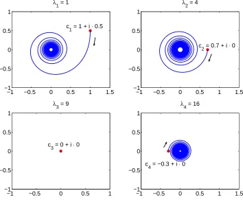
be viewed as a curve in the complex plane defined by zj(t) =hu(t), ϕji=rj(t) exp(iθj(t)).
Figure 2 shows an example of Γj(u0),j = 1,2,3,4,wherezj(t) = (t+ 1)−1/2cje−iλjtwith
cj = hu0, ϕji. For some chosen eigenvalues λj and Fourier coefficients cj we plotted zj(t)
on the time interval [0,∞). The trajectory t 7→ z(t) of the considered system in ℓ2(C) is
equal to a sequence t7→(zj(t))j∈N. In this way Figure 2 should indicate the projection of
the considered trajectory into C4.
−1 −0.5 0 0.5 1 1.5
−1 −0.5 0 0.5 1
λ1 = 1
c
1 = 1 + i ⋅ 0.5
−1 −0.5 0 0.5 1 1.5
−1 −0.5 0 0.5 1
λ2 = 4
c
2 = 0.7 + i ⋅ 0
−1 −0.5 0 0.5 1
−1 −0.5 0 0.5 1
λ3 = 9
c
3 = 0 + i ⋅ 0
−1 −0.5 0 0.5 1 1.5
−1 −0.5 0 0.5 1
λ4 = 16
c
[image:17.595.122.476.316.616.2]4 = −0.3 + i ⋅ 0
Figure 2. Projections Γj(u0) of Γ(u0),j = 1,2,3,4.
The following result describes some properties of the sequence ofd-dimensional Minkowski contents of curves Γj(u0) for d = 4/3, j ∈ N. Recall that if a set A ⊂ Rk is such that
Hence, since dimBΓj(u0) = 4/3 for all j, see Theorem 11(a) below, it has sense to
consider Md(Γ
j(u0)) for d= 4/3 only.
The sequence (Md(Γ
j(u0)))j will be called the Minkowski sequence associated to the
trajectory Γ(u0). More generally, for any trajectory Γ(u0) in L2(Ω) the corresponding
Minkowski sequence is (Mdj(Γ
j(u0)))j, where dj = dimBΓj(u0), provided the box
dimen-sion exists for eachj. The following result deals with properties of the Minkowski sequence associated to the trajectory of the NLS initial-boundary value problem (1) at the point of the bifurcation. As the cruical step in the proof of Theorem 11 we use the result of ˇ
Zubrini´c and ˇZupanovi´c [26, Theorem 6]. The simpler equivalent formulation can be found in [17, Theorem 3]. Because of the completeness, we briefly recall that result here.
Let Γ be a planar spiral defined in polar coordinates byr=f(θ), wheref(θ) is decreasing to zero as θ → ∞, such that f′(θ)/(θ−α)′ → p as θ → ∞, α ∈ (0,1), p > 0, and |f′′(θ)| ≤Cθ−α. Then dim
BΓ =d, where we defined d= 2/(1 +α), and
(28) Md(Γ) = pdπ(πα)−2α/(1+α)1 +α
1−α.
The asymptotic behaviour of the Minkowski sequence (Md(Γ
j(u0)))j for j → ∞ we
obtain using the following well known asymptotic result for the eigenvalues of −∆, due to H. Weyl. More precisely,
(29) λj ≃j2/N, j → ∞,
that is, there exist positive constants a and b such that for all j,a ≤λj/j2/N ≤b, see e.g.
Mikhailov [19, Section IV.1.5] or Davies [9, Theorem 6.3.1].
Theorem 11. Assume that a0 = 0 in (1), and γ1 6= 0.
(a) For any u0 ∈ L2(Ω) and j such that hu0, ϕji 6= 0 we have dimBΓj(u0) = 4/3.
Moreover,
(30) M4/3(Γj(u0)) = 3π1/3
λj|hu0, ϕji|2
|γ1| ku0k2L2 2/3
.
In particular,
(31) M4/3(Γj(u0))≤3π1/3
λj
|γ1|
2/3
,
and equality is achieved if and only if u0 ∈ span{ϕj}, u0 6= 0. Furthermore, we have the
following asymptotic behaviour
(32) max
u0∈L2(Ω)M
4/3
(b) For any u0 ∈H01(Ω), u0 6= 0, we have the following identity
(33)
∞ X
j=1
[M4/3(Γj(u0))]3/2 =
√ 27π
|γ1|
ku
0kH1 0 ku0kL2
2 . In particular, (34) ∞ X j=1
[M4/3(Γj(u0))]3/2 ≥
√ 27π
|γ1|
λ1,
and equality is achieved if and only if u0 ∈span{ϕ1}, u0 6= 0.
(c) For u0 ∈H01(Ω)∩H2(Ω), u0 6= 0, besides (33) we have the following identity:
(35)
∞ X
j=1
λj[M4/3(Γj(u0))]3/2 =
√ 27π
|γ1|
ku
0kH1 0∩H2 ku0kL2
2
,
and
(36) M4/3(Γj(u0)) =o(j−4/(3N)) as j → ∞.
In particular,
(37)
∞ X
j=1
λj[M4/3(Γj(u0))]3/2 ≥
√ 27π
|γ1|
λ21,
and equality is achieved if and only if u0 ∈span{ϕ1}, u0 6= 0.
Proof. (a) We consider the caseγ1 >0 (forγ1 <0 the proof is analogous). After eliminating
variable t from the system (18) one obtains
rj = |h
u0, ϕji|
ρ0
2γ1
arghu0, ϕji −θj
λj
+ρ−02
−1/2
=m(−θj +θ0)−1/2,
(38)
where θj → −∞, m = |h
u0, ϕji|
ρ0
s
λj
2γ1
, and θ0 is a constant. The expression (38) enables
to represent the spiral Γj(u0)⊂Cin polar coordinates (rj, θj) in a formrj =f(θj), where
f(θj) = m(θ0−θj)−1/2. Now, the expression (30) follows directly from the result of ˇZubrini´c
and ˇZupanovi´c [26, Theorem 6], which we briefly recalled at the beginning of this Section. We use the mentioned result in our situation by taking α= 1/2. Direct calculation gives
lim
θj→∞
f′(θ
j)
θj−1/2 =m,
The last claim follows from (31) and the Weyl asymptotic result (29) for the eigenvalues of −∆ subject to zero boundary data.
(b) Note that if hu0, ϕji = 0 then Γj = {0}, hence M4/3(Γj(u0)) = 0. ¿From this and
using (30), we obtain
(39) X
j
[M4/3(Γj(u0))]3/2 =
√ 27π γ1
ρ−02X
j
λj|hu0, ϕji|2.
Due to (13) this proves (33). Inequality (34) follows from the Poincar´e inequalityλ1ku0k2L2 ≤ ku0k2H1
0, and it is optimal since the constant λ1 is optimal.
(c) To prove (36), note that by (35) we haveλj[M4/3(Γj(u0))]3/2 →0 asj → ∞. Hence,
M4/3(Γ
j(u0)) = o(λj−2/3) = o(j−4/(3N)), where we exploited again the Weyl asymptotic
result (29).
The last claim follows from inequality ku0kH1 0∩H
2 ≥ λ1ku0kL2, which is an immediate
consequence of (13).
Remark 12. ¿From (30) we see that M4/3(Γ
j(u0)) → ∞ as γ1 → 0 in (1), provided
hu0, ϕji 6= 0. Another interesting consequence is that for any α6= 0,
M4/3(Γj(αu0)) =M4/3(Γj(v0)).
Hence, the mappingv0 7→ M4/3(Γj(u0)) is constant along rays through the origin inL2(Ω).
Since Γj(−u0) =−Γj(u0) for eachj, this mapping can be viewed as an even function defined
on the unit sphere S1 in L2(Ω).
Remark 13. Fora0 6= 0 all curves Γj(u0) are rectifiable near the origin, so that dimBΓj(u0) =
1. Moreover, M1(Γ
j(u0)) is equal to the length of the curve up to a multiplicative
con-stant independent of j and u0, see Federer [12, 3.2.39. Theorem], and its length depends
on the choice of t0 = t0j > tmin(u0). If d = dimBΓj(u0) > 1 (like in Theorem 11), then
Md(Γ
j(u0)) does not depend on the choice t0j due to excision property of d-dimensional
Minkowski content, see [25, Lemma 5.6(b)].
Remark 14. To see how the Minkowski sequence depends on the domain, let us denote by Ωε=εΩ the domain obtained from Ω by scaling using the factorε >0. To anyu0 ∈L2(Ω)
we assign u0ε ∈L2(Ωε) with u0ε(x) =u0(x/ε), and similarly for ϕjε. It is easy to see that
λjε =ε−2λj, and from this using (30) we obtain:
M4/3(Γj(u0ε)) = ε−4/3M4/3(Γj(u0)).
5. Box dimension of the trajectory
[11, Corollary 2.4(b)] and Tricot [23, see p. 121]. The main result of this section is given by theorem 17 and says that at the bifurcation valuea0 = 0 the box dimension of trajectories
of (1) viewed near the origin in L2(Ω) (or near the origin of ℓ
2(C) for (3)) has a jump.
More precisely, for u0 6= 0 the mapping a0 7→ dimBΓa0(u0) is discontinuous at a0 = 0, where Γa0(u0) is the trajectory of (1) corresponding to u0 and a0.
5.1. Multiple spirals. For a given trajectory Γ(u0) in L2(Ω) we define its box dimension
via finite-dimensional approximations:
(40) dimBΓ(u0) = lim
k→∞dimBΠk(Γ(u0)),
where Πk is the orthogonal projection of the Lebesgue space onto span{ϕ1, . . . , ϕk}, or
equivalently, from ℓ2(C) onto Ck, corresponding to the first k components of ℓ2(C). The
above limit exists due to the monotonicity property of box dimension, see Falconer [11, p. 37].
By the multiple spiral(or n-spiral) Γ2N we mean a curve in CN =R2N defined by
(41) Γ2N ={(t−α1eiλ1t, . . . , t−αNeiλNt)∈CN: t≥t0},
where t0 > 0. The following result will be fundamental for the computation of box
di-mension of trajectories of problem (1). Its consequence is that box didi-mension of multiply oscillating trajectories in CN is always less then 2. The claim extends the formula of box
dimension of planar spirals due to Tricot [23, p. 121] to oscillating curves inCN. Since the
result seems to be interesting for itself, we state it in a slightly more general form.
Theorem 15. Let αk > 0 and λk 6= 0 be given numbers, k = 1, . . . , N. Then the
corre-sponding multiple spiral Γ2N has box dimension
(42) dimBΓ2N = max
n
1, 2
1 + minkαk
o
.
The curve Γ2N is Minkowski nondegenerate if and only if minkαk 6= 1. It is rectifiable if
and only if minkαk >1.
Proof. (a) We assume without loss of generality thatα1 is minimal among allαi. Let Γ2 be
the curve inCdefined byt7→t−α1eiλ1t. Let us introduce the mapping F : Γ
2 →Γ2N in the
following way. First, we view the curves Γ2 and Γ2N as subsets ofR2 and R2N respectively,
and define (writing zk =xk+iyk):
(43) F(x1, y1) = (x1, y1, f2(x1, y1), g2(x1, y1), . . . , fn(x1, y1), gn(x1, y1)),
where
fk(x1, y1) =
λ−11arctany1 x1
−αk
coshλkλ−11arctan
y1
x1
i
,
gk(x1, y1) =
λ−11arctany1 x1
−αk
sinhλkλ−11arctan
y1
x1
i
for 2 ≤k ≤N. It is easy to check that F maps Γ2 bijectively onto Γ2N. Let us estimate
the expression ∂fk
∂x1
= C1
arctany1 x1
−αk−1 y1
x2 1+y12
coshλkλ−11arctan
y1
x1
i
+C2
arctany1 x1
−αk
sinhλkλ−11arctan
y1
x1
i y1
x2 1+y12
along Γ2. Here C1 and C2 are real constants. It follows:
(44)
∂fk
∂x1
≤
C(tα1−αk−1+tα1−αk) =O(tα1−αk), t→ ∞.
Since α1 ≤ αk the function ∂f∂xk1 is bounded by a constant along Γ2. Similarly for ∂f∂yk1, ∂g∂xk1
and ∂gk
∂y1. This proves that the mappingF is Lipschitzian. It is easy to see that the inverse
F−1 : Γ
4 → Γ2 is the projection of Γ4 onto Γ2, which is also Lipschitzian. Hence, F is a
bilipschitz function, so that we may use Falconer [11, Corollary 2.4(b)] with Tricot [23, see p. 121] to obtain that:
dimBΓ2N = dimBF(Γ2) = dimBΓ2 = max
n
1, 2 1 +α1
o
.
Minkowski nondegeneracy of Γ2N for α1 ∈(0,1) follows from [27, Theorem 1], since Γ2
is Minkowski nondegenerate, and moreover Minkowski measurable, see [26, Corollary 2], and Γ2N is lipeomorphic (i.e. bilipshitz equivalent) to Γ2. If α1 ≥ 1, then dimBΓ2N =
dimBΓ2 = 1. For α1 = 1 we have M1(Γ2N) =∞ since nonrectifiability of Γ2 implies that
Γ2n is also not rectifiable.
Remark 16. The condition on αi to be positive is essential. Indeed, if N = 2 and
α1 =α2 = 0, then we obtain the curve on the 2-torus, and assuming thatλ1/λ2 is rational
we obtain that the curve is periodic, hence its box dimension is 1. Therefore, formula (42) does not hold in this case. A more general formulation of the first part of the theorem is as follows: if αj ≥0 for all j and the set J ={j :αj >0, λj 6= 0} is nonempty, then
dimBΓ2N = max
n
1, 2
1 + min{αk:k ∈J}
o
,
and analogously for the second part.
Now, using the result given by theorem 15 we are able to show that at the bifurcation value a0 = 0 the box dimension of trajectories of (1) viewed near the origin in L2(Ω) (or
near the origin of ℓ2(C) for (3)) has a jump.
Theorem 17. Assume that u0 6= 0 and γ ∈ R\ {0}. Let Γ(u0) be the trajectory of (1)
viewed in a bounded neighbourhood of the origin. If a0 = 0 then dimBΓ(u0) = 4/3. If
Proof. We consider the case of γ =γ1+iγ2 with γ2 = 0 and γ1 >0 (for γ1 <0 the proof
is analogous). The case when γ1 6= 0 and γ2 6= 0, see (18), can be treated with slight
modifications.
The projection of solution u(t) defined by (19), viewed in ℓ2(C), onto its first n
compo-nents, defines the following curve in CN:
Γ′
2N. . . t7→uN(t) =
1
q
2γ1t+ku0k−L22
(c1e−iλ1t, . . . , cNe−iλNt)
where cj = hkuu00k,ϕji
L2, t ≥ t0 with t0 large enough. We assume for simplicity that cj 6= 0 for allj. It is natural to define the curve
Γ2N. . . t7→vN(t) =t−1/2(e−iλ1t, . . . , e−iλNt).
The mapping G : Γ′
2N → Γ2N defined by G(uN(t)) = vN(t) for all t ≥ t0 > 0, is clearly
bilipschitzian, hence dimBΓ′2N = dimBΓ2N. The claim follows from Theorem 15. The case
when cj 6= 0 for at least one j, is treated with minor modifications of the above proof.
If a0 6= 0, then all components zj(t) are rectifiable, hence any finite-dimensional
pro-jection πk(Γ0) is rectifiable, where πk : ℓ2(C) → Ck it the natural projection onto the
first k components of ℓ2(C). This implies that dimBπk(Γ0) = 1 for each k, and the claim
follows.
As we saw before, assuming that a0 = 0 and γ1 6= 0, the natural projection of any
trajectory Γ(u0) into j-th component, that is, into the eigenspace spanned by ϕj, can be
viewed as a curve in the Gauss plane either of box dimension 4/3 if hu0, ϕji 6= 0 (in this
case the projection is a spiral), or zero if hu0, ϕji= 0 (in this case the projection is simply
a point).
6. Applications
In this section we introduce the notion of spiral chirp. The aim is to study the box dimension of spiral chirps and associated trajectories of NLS problems with different non-linearities. To achieve this goal, we shall use the results on box dimensions of trajectories obtained in previous sections. Finally, in Subsection 6.3 we show that a class of planar polynomial dynamical systems can be interpreted in terms of a NLS problem of nonlocal type.
6.1. Box dimension of spiral chirps. Results on box dimension of trajectories of NLS initial-boundary value problem (1) obtained in the previous section can be used in order to calculate the box dimension of some other curves, for example spiral chirps. More precisely, in the preceding subsection we have studied box dimension of projections of Γ0
consider projections onto R2N−1. The basic model in R3 is the curve that we call spiral
chirp:
(45) Γ =n(t−αcost, t−αsint, t−αcost)∈R3: t≥t0o,
with α∈(0,1). A more general model could be (α, β)-spiral chirp:
(46) Γ3 =
n
(t−αcos(λ1t), t−αsin(λ1t), t−βcos(λ2t))∈R3: t ≥t0
o
,
for fixed positive α,β, t0, andλj 6= 0,j = 1,2. Of course, box dimension of Γ3 will remain
the same if we replace the last component with t−βsinλ 2t.
Theorem 18. Let α and β be fixed positive numbers such that either
α ≤β, or β ≤α <1, or 1< β ≤α.
Furthermore, assume that λ1, λ2 are nonzero real numbers, andt0 >0. Then for the spiral
chirp Γ3 defined by expression (46) we have:
(47) dimBΓ3 = max
n
1, 2
1 + min{α, β}
o
.
The curve Γ3 is rectifiable if and only if min{α, β}>1.
Proof. Due to the simplicity we assume that λ1 =λ2 = 1.
Firstly, we consider the case α≤β.
Note that we have natural projections π43 : Γ4 → Γ3 and π32 : Γ3 →Γ2, where Γ2 ⊂ R2
is the spiral defined by t 7→ z1(t) = t−αeit, and Γ4 ⊂ R4 is 2-spiral defined by t 7→
(z1(t), z2(t)), with z2(t) = t−βeit. Hence, since the projections are Lipschitzian, using
known box dimensions of Γ2 (see Tricot [23, see p. 121]) and Γ4 (see Theorem 15), it
follows
dimBΓ2 = dimBπ32(Γ3)≤dimBΓ3 = dimBπ43(Γ4)≤dimBΓ4.
Now, the desired result follows directly since dimBΓ2 = dimBΓ4 =d, where we used the
notationd= max{1,2/(1 +α)}.
Next, we consider the case when β ≤α <1.
Since the natural projection π43 : Γ4 → Γ3 is Lipschitzian, it follows that dimBΓ3 ≤
2/(1 +β). To prove the opposite inequality, it suffices to construct a surjective Lipschitz mapping F : Γ3 →Γ2, where Γ2 is described by r=ϕ−β, since then
2
1 +β = dimBΓ2 = dimBF(Γ3)≤dimBΓ3. In this way let us construct an auxiliary spiral Γ′
2 defined by
with positive parameters a and b to be chosen later. It is easy to see that the mapping F = (F1, F2) where
F1(x, y) =
arctany x
−a
cosarctany x
b
,
F2(x, y) =
arctany x
−a
sinarctany x
b
maps Γ3 onto Γ′2. Now, it remains to to find a and b such that F is Lipschitzian on Γ3.
First, since ∂x∂ (arctan(y/x)) =O(tα), and similarly ∂
∂y(arctan(y/x)) =O(t
α), whent → ∞
it follows that
∂F1
∂x =O(t
α−a−1) +O(tα−a+b−1),
and similarly for the remaining first order derivatives ofF1 andF2. Finally, in order to have
the boundness of|∂Fi
∂x|and| ∂Fi
∂y|, it suffices to impose thatα−a−1≤0 andα−a+b−1≤0.
The curve Γ′
2is defined byr=ϕ−a/b, and sincea/b≤1, we have dimBΓ′2 = 2/(1+(a/b)),
see Tricot [23, p. 121]. In order to have dimBΓ′2 = 2/(1 +β) we choose a and b so that
β = a/b. To have b−a≤ 1−α we impose even b−a = 1−α. ¿From a =βb we obtain b−a=b(1−β) = 1−α, hence b = (1−α)/(1−β), and from this a=β(1−α)/(1−β). This choice for a and b satisfies all the requirements.
Finally, the proof for the case 1< β ≤α goes similarly to the previous considerations. At the end of the proof, let us consider the rectifiability in the case when min{α, β}>1. The spiral Γ2 is rectifiable, as well as the graph of the chirp z1(t) = tβcost−1 for t near
zero, corresponding to the third component of Γ3. In this case the curve Γ3 is rectifiable
as well. Indeed, since z1(t) has local extrema for tk such that tk−1/β = ±π2 + 2kπ, then
tk ≃k−β ask → ∞, hence,
(48) l(Γ3)≤l(Γ2) + 2
X
k
|z1(tk)| ≤l(Γ2) +c
X
k
k−β <∞,
since β > 1. This implies that dimBΓ3 = 1. The first inequality in (48) can be justified
by isometrically transforming Γ3 onto the chirp defined in rectangular coordinates, defined
on the interval of length of the spiral Γ2.
On the other side, if min{α, β}<1 then from (47) we see that dimBΓ3 > 1, hence, Γ3
is not rectifiable. In the case when min{α, β}= 1, let us consider the following two cases: (i) If α = 1, the spiral Γ2 defined by z(t) = t−1eit is nonrectifiable. Since M1(Γ3) ≥
M1(Γ
2) =∞, the same holds for Γ3.
(ii) If β = 1, then the chirp Γ′
2 is not rectifiable. Using a suitable parametrization of Γ3
and the fact that F(Γ3) = Γ′2 with a Lipschitzian map F, since Γ′2 is nonrectifiable then
also Γ3 is nonrectifiable.
Corollary 19. LetΓ2N ⊂R2N,N ≥1, be a multiple spiral defined by (41), with0< αk <1
andλk6= 0, k= 1, . . . , N. Let e1, . . . , e2N be the canonical orthonormal base inR2N. Then
for the multiple spiral chirp Γ2N−1 obtained by projecting Γ2N into (2N −1)-dimensional
subspace of R2N spanned by any2N −1 vectors from the base, we have
dimBΓ2N−1 = dimBΓ2N =
2 1 + minkαk
.
6.2. Hopf bifurcation for other types of nonlinearities. Up to now we studied the initial-boundary value problem for Schr¨odinger equation
ut=i∆u−γuV(kukL2(Ω)), (49)
where Ω ⊂ RN and γ = γ1 +iγ2 ∈ C. More precisely, we considered the nonlinearity
V(ρ) = ρ2 +a
0, where a0 was a real bifurcation parameter. In this section we consider
some polynomial types of nonlinearity given by the expression
(50) V(ρ) =ρ2l+al−1ρ2(l−1)+· · ·+a1ρ2+a0,
where ai, i = 0, . . . , l−1 are prescribed real parameters. The NLS equation (49)
corre-sponds to thestandard generic generalized Hopf bifurcation, see Takens [22], also called the standard Hopf-Takens bifurcation. The following result extends Theorem 17.
Theorem 20. Let Γ(u0) be a part of trajectory of (49) near the origin with V(ρ) defined
by (50), such that u0 6= 0, γ2 = 0 and γ1 = 06 . Assume that k := min{j : aj 6= 0} ≥ 1.
Then
(51) dimBΓ(u0) =
4k 2k+ 1.
Proof. The proof uses the idea of the proof of Theorem 17, together with the proof of [26, Theorem 9(b)]. Hereα= 1/(2k), so that the box dimension is obtained from Theorem 15. Up to now we studied trajectories with spiral components zj(t) converging to zero with
equal rateα >0, that is,|zj(t)| ≃t−α ast→ ∞, for allj, see for example expressions (45)
or (46). Next, we are interested in dynamical systems yielding solutions in which spiral components converge to zero with different rates.
A. As the simplest model we consider a polynomial system in inC2, defined by
(52) z˙j =−iλjzj−
1 4mj
zj(|z1|2m1 +|z2|2m2 +a0), j = 1,2,
wheremj are fixed positive integers anda0is the real bifurcation parameter. It is easy to see
that fora0 <0 an attracting invariant setS(a0) is born, defined by|z1|2m1+|z2|2m2 =−a0,
diffeomorphic to the unit 3-sphere inC2. Each trajectory starting in the point (z10, z20)∈ S(a0) is contained in the torus |z10|S1 × |z20|S1 (provided that both components zj0 are
Assume that a0 = 0 and let z(0) = (z01, z02)∈ C2 be a given initial value, z(0)6= 0. It
can be shown that the unique solution z(t) = (zj(t)) of system (52) is given by
zj(t) =|z0j|(t+ 1)−1/(2mj)exp(−iλjt+iargz0j), j = 1,2.
Here zj(t) is a spiral converging to zero with rate αj = 1/(2mj). Assume that both
z01 and z02 are different from zero. According to Theorem 15 the box dimension of the
corresponding trajectory Γ4 ={(z1(t), z2(t))∈C2 :t ≥t0 >0} is equal to
dimBΓ4 =
2
1 + 0.5 max{m1, m2}−1
. (53)
System (52) is a special case of the following Schr¨odinger equation:
(54) ut =i∆u−F(u),
with initial and boundary values as in (1), and
F(u) = |hu, ϕ1i|2m1 +|hu, ϕ2i|2m2 +a0
2
X
j=1
1 4mjh
u, ϕjiϕj(x),
with scalar products inL2(Ω). System (52) is obtained from (54) by considering solutions
of the formu(t, x) =z1(t)ϕ1(x) +z2(t)ϕ2(x), whereϕ1 andϕ2 are defined in the subsection
1.2.
B.Various extensions of (52) and (54) are possible, like for example a cyclic polynomial system in R2k, which we view as a bifurcation problem inCk:
˙
z1 = −iλ1z1−
1 4m1
z1(|z1|2m1 +|z2|2m2 +a0)
˙
z2 = −iλ2z2−
1 4m2
z2(|z2|2m2 +|z3|2m3 +a0)
.. .
˙
zk = −iλkzk−
1 4mk
zk(|zk|2mk+|z1|2m1 +a0).
(55)
For a0 < 0 an invariant set S(a0) is born in Ck defined by |z1|2m1 +|z2|2m2 = |z2|2m2 +
|z3|2m3 =· · ·=|zk|2mk+|z1|2m1 =−a0, which is a subset the surface defined byPj|zj|2mj =
−k2a0, diffeomorphic to the (2k−1)-sphere in Ck.
Here system (55) again has the form of the Schr¨odinger equation (54), but with
F(u) =
k
X
j=1
1 4mjh
u, ϕji |hu, ϕji|2mj +|hu, ϕj+1i|2mj+1+a0
ϕj(x),
and the summation of indices in j + 1 is taken modulo k. Here we consider solutions of the form u(t, x) =Pk
For a0 = 0 and any prescribed initial value z(0) = (z0j) ∈Ck it can be shown that the
unique solution is the curve Γ2k ={(z1(t), . . . , zk(t))∈Ck:t ≥0} of (55), defined by
(56) zj(t) =|z0j|(t+ 1)−1/(2mj)exp(−iλjt+iargz0j), j = 1, . . . , k.
Using Theorem 15 with αj = 1/(2mj) we obtain the following result.
Corollary 21. Let mj be positive integers and a0 = 0. For any trajectoryΓ2k of (55) such
that z(0) = (z01, . . . , z0k)6= 0we have
dimBΓ2k=
2
1 + 0.5 max{mj :z0j 6= 0}−1
.
C.Now we would like to construct a NLS Cauchy problem possessing trajectories of box dimension equal to two. Let us consider the Schr¨odinger equation of the form (54) such that
(57) F(u) = ∞ X
k=1
(|hu, ϕ2k−1i|2m2k−1 +|hu, ϕ2ki|2m2k +a0) 0
X
j=−1
1 4m2k+jh
u, ϕ2k+jiϕj(x),
where mj is a prescribed sequence of positive integers. First, if u ∈ L2(Ω) then also
F(u) ∈ L2(Ω). Indeed, the expression in the round brackets is bounded by a constant
M =M(u, a0, m1, m2, . . .) independent of j, since hu, ϕjiconverges to zero. Hence,
kF(u)k2L2 ≤M2
∞ X
k=1 0
X
j=−1
1 4m2k+jh
u, ϕ2k+jiϕj
2
L2
≤ M
2
16 kuk
2 L2.
It can be shown that if u(t) = P
jzj(t)ϕj is a solution of (54) with initial value u(0) =
u0 ∈L2(Ω), then zj(t) is uniquely determined, and
zj(t) =|hu0, ϕji|(t+ 1)−1/(2mj)exp(iλjt+iarghu0, ϕji), j ≥1.
Denote by Γ(u0) the trajectory in L2(Ω) corresponding to t ≥ 0. Using the definition of
dimBΓ(u0) in (40) and Theorem 15 we obtain the following result.
Corollary 22. Let a0 = 0. Let u(t) be the solution of (54) with F(u) defined by (57), and
a0 = 0, satisfying initial condition u(0) =u0 ∈L2(Ω). Then
dimBΓ(u0) =
2
1 + 0.5 sup{mj :hu0, ϕji 6= 0}−1
. (58)
In particular, if mj → ∞ as j → ∞, and hu0, ϕji 6= 0 for infinitely many j’s, then
6.3. Box dimension of trajectories of some nonintegrable Schr¨odinger problems.
Many dynamical systems important for applications, like for example Li´enard systems, weakly damped systems etc., are not explicitly solvable. However, in spite of their nonin-tegrability it is possible to get the information about the box dimension of corresponding trajectories, see [30] for some examples. Here, using the connection between the nonlinear system of ODE’s and the Schr¨odinger equation pointed out already in Section 1.2, we would like to study the box dimension of trajectories of some nonintegrable Schr¨odinger evolution problems. For this purpose let us consider the following polynomial planar system:
˙
x=f(x, y) = λ1y+p(x, y)
˙
y=g(x, y) =−λ1x+q(x, y),
(59)
where we define p(x, y) = f(x, y)−λ1y and q(x, y) = g(x, y) +λ1x. Here λ1 is the first
eigenvalue of the −∆|H1 0∩H
2 corresponding to an open and bounded domain Ω⊂RN. An initial point in the phase space is prescribed byx(0) =x10andy(0) =y10. Naturally, we say
that the system (59) is equivalent to (54) if there is a bijection between the corresponding solution sets. In this sense it is easy to see that the problem (59) is equivalent to Schr¨odinger equation (54) with F: Cϕ1 →Cϕ1 defined by
(60) [F(u)](ξ) =p(hReu, ϕ1i,hImu, ϕ1i) +iq(hReu, ϕ1i,hImu, ϕ1i)
ϕ1(ξ), ξ∈Ω,
and with initial functionu(0) =z01ϕ1, wherez01=x10+iy10 ∈C. Note that the nonlinear
term F(u) is of nonlocal type, i.e. F it is not defined in pointwise manner, but via scalar products, that is, by means of two integrals. The solution of (54) in this case has the form u(t, x) =z(t)ϕ1(x), where z(t) =x(t) +iy(t), and the components satisfy (59). Note that
(54) is of nonlocal type, and in general not explicitly solvable. Moreover, it is interesting that the study of any system of ODE’s can be considered as the study of a Schr¨odinger problem.
Proposition 23. Any Cauchy problem for the system x˙ = f(x), where x ∈ Rn and
f:Rn →Rn is a Lipschitz function, can be naturally interpreted as a Schr¨odinger problem
of the form (54), with F(u) written explicitly, see (62) below.
Proof. We can assume without loss of generality thatn is even, n = 2k (if n= 2k−1, we can add a new trivial equation ˙x2k = 0, x2k(0) = 0). Now the system can be written in the
form
(61) x˙j =fj(x, y)
˙
yj =gj(x, y)
j = 1, . . . , k
wherex, y ∈Rk. Definingzj =xj+iyj and pj(x, y) =fj(x, y)−λjyj,qj(x, y) =gj(x, y) +
λjxj, j = 1, . . . , k, where λj are the first k eigenvalues of −∆ (counting the multiplicity)
defining u(t, ξ) = P
jzj(t)ϕj(ξ) we easily obtain (54), where the operator F: Xk → Xk,
Xk= spanC{ϕ1, . . . , ϕk} ⊆L2(Ω), is defined by
(62)
F(u)
(ξ) =
"
F