THE SPACE-SCALE CUBE: AN INTEGRATED MODEL FOR 2D POLYGONAL AREAS
AND SCALE
Martijn Meijers and Peter van Oosterom
Delft University of Technology
OTB Research Institute for the Built Environment Section GIS technology
Jaffalaan 9, 2628 BX Delft, The Netherlands [email protected], [email protected]
Commission IV/WG8
KEY WORDS:Multiresolution, Theory, Generalization, Simplification, Visualization, GIS
ABSTRACT:
This paper introduces the concept of a space-scale partition, which we term thespace-scale cube– analogous with the space-time cube (first introduced by H¨agerstrand, 1970). We take the view of ‘map generalization is extrusion of 2D data into the third dimension’ (as introduced by Vermeij et al., 2003). An axiomatic approach formalizes the validity of the partition of space in three dimensions (2D space plus 1D scale). Furthermore the paper provides insights in how to: 1. obtain valid data for the cube, 2. obtain a valid 2D polygonal map at variable scale from the cube and 3. which other possibilities the cube brings for obtaining maps having different map scales over their domain (which we termmixed-scalemaps).
1 INTRODUCTION
For displaying geographic information amapis an often used tool to portray characteristics of some geographic phenomena. User interfaces in Geographic Information Systems (GIS) mainly use maps to let users interact with the geographic phenomena under study. An important feature of maps is that they show topologi-cal relationships between geographic objects, which can be made explicit in data structures (Hoel et al., 2003; van Oosterom et al., 2002). As limited space is available for portrayal on any medium (e. g. paper, screen, projector), it is not sensible to show repre-sentations of geographic objects with all their details. It is better to adjust the level of detail to the amount of space available (i. e. apply generalization for smaller map scales).
This paper introduces the concept of a space-scale partition, which we term the space-scale cube(analogous with the space-time cube proposed by H¨agerstrand, 1970). Map generalization of 2D polygonal regions is seen as extrusion into the third dimension (similar to Vermeij et al., 2003, where this idea was introduced first). We formalize what we consider valid data for this cube. The focus is on maps of polygonal regions in planar partitions, because for a lot of applications polygons are a useful building block for modelling, amongst others, administrative units, land use, soil maps, topographic maps, zoning plans, etcetera. The space-scale cube permits us to obtain an integrated 3D model, composed of both the dimensions of 2D space and 1D scale (or level of detail). From the 3D cube it is possible to extract a consis-tent 2D map at variable scale (as the cube is one integrated model of space and scale any derived slice from the cube must again be a valid 2D planar partition). The formalization stems from re-searching the topological Generalized Area Partitioning (tGAP) structures (Meijers et al., 2009; van Oosterom, 2005) and the de-sire to express what is valid data stored in the structures. The cube encodes both a description of space at variable map scale as well as the generalization process (transitions in scale dimension).
The questions that we explore in this paper are the following:
• How can valid, polygonal regions forming a valid partition (in 2D) be transformed in a 3D space-scale cube and when do we consider a space-scale cube valid?
• What possibilities does the cube offer us to obtain a consis-tent 2D map?
Section 2 introduces the primitives we use for modelling 2D space, describes what we term a valid polygon and how we build a par-tition of 2D space. Section 3 explains our vision of how the inte-grated 3D space-scale cube encodes both 2D space and 1D scale at the same time. Section 4 describes how the cube can be used for deriving a 2D polygonal map. Section 5 concludes the work and suggests further research.
2 A VALID 2D DESCRIPTION OF SPACE
To obtain input for a valid 3D space-scale cube (SSC), we first give a formal description of data for a 2D planar partition. It is not the intent to redefine the common notion of what is a valid polygon (c. f. van Oosterom et al., 2003), but to give a formal basis for input data on which we can run a generalization process for deriving a valid SSC (and later on the formal description will be extended for the 3D SSC).
In the formal description we use notions from set theory and borrow ideas from the formalization approach that Erwig and Schneider (1997) describe. Keep in mind that here we aim at a formal and reasonably abstract model, but that this model later will have to be translated in data structures in a computer; an im-plementation of those data structures are not the main purpose now, but sometimes we will look forward and act if we were al-ready targeting an implementation of the SSC.
2.1 Spatial building blocks
Definition 1. Given ak-dimensional Euclidean spaceRk, called X.
Definition 2. InX, we distinguishk+ 1distinct types of primi-tives.
Definition 3. We name ai-dimensional primitivepi
, whereiis: 0a node (p0
),1a edge (p1
),2a face (p2
) and3a volume (p3
).
Definition 4. The primitivespi
arenon-emptysubsets of points ofMi
, that ispi ⊂Mi
. HereMi
is asupporting subspaceof dimensioniwithMi⊂ Xand where for the dimensioniholds:
0 ≤ i ≤ k. Primitivespi areconnectedand openin Mi (or relatively openinX). Open means that for any given pointxin a primitivepi, there exists a real numberǫ >0, such that, given any other pointyinpi, which has an Euclidean distance smaller thanǫtox,yalso belongs top(theǫdistance defines an open ball with infinitesimal small radius). Connected means that for every pair of pointsx, y ∈ piholds that there is always a path within the interior ofpi
that connects the two points.
What needs to be true for all primitivesPinX (note thatPis used to name the set with all primitivespthat coverX):
Axiom 1. Xis not empty;X 6=∅.
Axiom 2. Every primitivepis part ofX;∀p ∈ P : X ∩p = p∧p6=∅.
Axiom 3. All primitives are pairwise disjoint, i. e. no points are shared between primitives;∀i, j∈ P, i6=j:i∩j=∅.
Axiom 4. The union of all primitivesPtotally coversX;∪pp∈
P=X.
Based on definitions and axioms, what also has to be true for primitives is that:
Theorem 1. There is at least onek-dimensional primitivepin X.
Proof. Xis totally covered (Axiom 4) andX 6=∅(Axiom 1) and for implementation finite primitives are used⇒ ∃pk
∈ X
Remember thatkis the highest dimension, that is, the dimension of the embedding spaceX. In theory it is possible to coverX with an infinitely refined space filling curve.
2.2 Map objects and labels
To represent real world objects, we now introduce map objects that we term zones. We define the names of thei-dimensional zones as follows.
Definition 5. We term ai-dimensional zoneωwhere i = 0a vertex (ω0
),i = 1a polyline (ω1
),i = 2a polygon (ω2
) and i= 3a polyhedron (ω3
).
To discriminate a zone from all other zones, we introduce the concept of labelling zones. A label is meant for giving a proper identity to the zones, i. e. a label is a globally unique identifier.
Axiom 5. All zones have a globally unique labelλ.
Furthermore, we require that zones form a closed and connected entity:
Definition 6. All zones are closed and connected.
Apart from all real world objects that are mapped, we also have a zone that represents the unmapped domain, a zone that represents the space outside the mapped domain:
Definition 7. A zone with label⊥represents the space ‘outside’ the mapped domain.
Note that the ‘outside’ zone is allowed to have multiple parts: exactly one part that is not completely bounded (in the direction of infinity) and optionally other parts that are completely bounded (e. g. this is the case with exclaves of the ‘outside’ zone).
To represent a zone inX, we associate the zones with the primi-tives inX:
Axiom 6. A zoneωis formed by the union of its associated prim-itives. These primitives have the sameandlower dimensions as ωi. Ai-dimensional zoneωis formed byi∪i−1∪. . .∪0 -dimensional primitives.
To end up with valid zones, we label all primitivesPbased on the labels that the zones have:
Axiom 7. For a zoneωwe require that there is exactly one prim-itivepwith the same labelλand same dimension as the zone.
And we require that a labeling procedure to give labels to the primitives inXis carried out as follows:
Axiom 8. All primitives inX have to be labelled following this recipe:
1. All primitives start with an empty label set.
2. For every zoneωi, add its labelλto all associated primitives of dimensioni.
3. Add to each remaining primitivep, that has a dimensioni smaller than that of its associated zone(s) and has not been labelled, the set of labels of the points that are inside an epsilon discǫcentered on the points ofp.
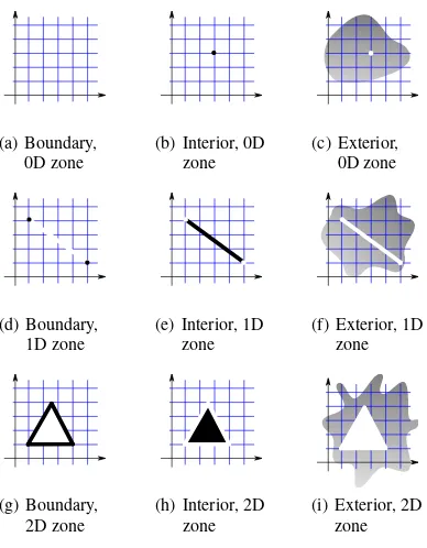
After labelling we can derive the interior, exterior and boundary primitives of ani-dimensional zoneω(Figure 1 illustrates these concepts):
Definition 8. Interior (ω◦) of a zone: the associatedi-dimensional
primitive that has a label set with exactly one label and which is equal to the label of the zone.
Definition 9. Boundary (∂ω) of a zone: the set of< i-dimensional primitives that have the label of the zone in its label set.
Definition 10. Exterior (ω−) of a zone: all primitives inXnot
having the label of the zone in their label set.
(a) Boundary, 0D zone
(b) Interior, 0D zone
(c) Exterior, 0D zone
(d) Boundary, 1D zone
(e) Interior, 1D zone
(f) Exterior, 1D zone
(g) Boundary, 2D zone
(h) Interior, 2D zone
(i) Exterior, 2D zone
Figure 1: Boundary, interior, exterior for 0D, 1D and 2D zones (intent illustrated in black/dark grey). Note that a 0D zone does not have a boundary (by definition there will not be any primitives with dimension<0).
{A}
{⊥}
{A,⊥}
{⊥}
(a) Spike in boundary.
{B}
{B,⊥} {B}
{⊥}
(b) Loose-lying segment in interior.
Figure 2: Degenerate cases will be prevented by correct labelling.
Axiom 9. For a spaceX wherek = 2the primitivesP ∈ X have to be labelled as follows:
• p0
: three or more different labels
• p1
: two different labels
• p2
: exactly one label
It has been defined how a zone is represented and is composed by its associated, unambiguously labelled primitives. Loose bound-ary parts and spikes, such as shown in Figure 2, are prevented, as those segments would only have one distinct label and as these degeneracies do not add any extra information (e. g. it is already known that that part of the space belongs the polygon) it is use-ful to prevent these situations. As a final remark, note that this set of statements allows holes to exist in polygonal regions and multi-part polygons are not allowed (Axiom 7).
2.3 A valid 2D planar partition
For a valid 2D planar partition we will not allow zones with lower dimension thankto exist, which means that whenk= 2we only allow polygons.
Axiom 10. ForX, we only allowk-dimensional zones.
We also state that zones are not allowed to overlap each other in their interior:
Axiom 11. Zones are only allowed to share associated primitives in their boundary and not in their interior:∀ω1, ω2 ∈Ω, ω1 6=
ω2:pk1∩p
k
2 =∅withΩthe set of all zones.
From the definitions and axioms, we can now derive that the in-teriors of zones are unambiguously labelled.
Theorem 2. The interior of a zone,pkprimitive, is labelled with exactly one label.
Proof. Following from that primitives are not allowed to over-lap (Definition 3), that for every zone there is a labelled primi-tive having the same dimension (Axiom 7) and that there are no shared primitives between zones (Axiom 11) follows that the in-terior of a zone has to be labelled with exactly one label.
2.4 Targeting implementation
To make it easier to translate the abstract model to a suitable data structure for a computer and to be able to define incidence and adjacency (see next subsection), in addition to Axiom 6 where we state that a zone is a collection of primitives, we add:
Axiom 12. For every dimensioni∈ {0, . . . , k}there is at least one primitive associated with zoneω.
This then does translate nicely to data-structures, like DCEL, to encode the incidence relationships of the boundaries (but where the interior point set is not represented explicitly). From the topology point of view a closed ring of a single island zone does not have a node (p0
). From the implementation point of view it is nice if every edge (p1
) starts and ends at a node (twop0
, possi-bly equal). We will have to add nodes where previously this was not the case and it it is necessary to replace Axiom 9 (as such a node has just 2 labels and not 3 or more labels as for topologically defined nodes):
Axiom 13. For a planar partition wherek = 2, the primitives P ∈ X have to be labelled as follows:
• p0
: two or more labels
• p1
: exactly two labels
• p2
: exactly one label
As last requirement, we will define that subsets of points in an edge have to be straight in geometrical sense (not curved).
Definition 11. Connected subsets of points in an edge (p1
(a) Planar partition of four
(b) Associated primitives of four 2D zones (polygons).
(c) Incidence graph for the primitives representing the four polygons in (a) and the associated primitives in (b). The 2 polygons for which their interior is represented byf0andf1are 1-adjacent, as two paths exist that overlap (and the highest dimensional primitive in the overlap is at the 1-dim level, therefore 1-adjacent),
f0, e1, n0andf1, e1, n0.
Figure 3: Incidence and adjacency can be defined by drawing a graph of how the composing primitives for zones are related.
2.5 Incidence and adjacency
From how the primitives are associated with zones, we can obtain a Directed Acyclic Graph (DAG), termed the incidence graph (L´evy and Mallet, 1999). Figure 3(c) shows the incidence graph for the primitives drawn in Figure 3(b). The highest dimensional primitives will form the top nodes of this directed graph. Edges in the graph represent how ak-dimensional zone is composed of primitives. Primitives having the same dimension are drawn on the same level in the tree structure. Based on the drawing of the DAG, we can defineincidencerelationships of primitives and adjacencyrelationships of zones. With respect to incidence, we can also define the termdegreeof a primitive as the number of incoming graph edges within the DAG.
Incidence Two primitives are said to beincident, when there ex-ists a path between two primitives in the DAG.
Adjacency If two zones have paths in the incidence graph, that partly overlap, and the highest dimensional overlapping prim-itive is at leveli, then the two zones are said to bei-adjacent. Furthermore, these two zones will be said to bestrongly con-nectedwheniis exactly one dimension lower than the zone, that is,i=k−1.
3 FROM 2D SPACE AND 1D SCALE TO 3D SSC
As limited space is available for portrayal on any medium (e. g. paper, screen, projector), it is not always sensible to show repre-sentations of geographic objects with all their details. It is better to adjust the level of detail to the amount of space available (i. e. apply generalization for smaller map scales). This section puts forward how we see that the result of a generalization process of a 2D map can be represented by a description of 3D space and what statements we need to add to the statements of the previous section, to enforce a valid partition in 3D.
3.1 Generalization operations
A generalization process is often seen as a process, that for an in-put map outin-puts a completely new and independent derived map
with lower level of detail (Mackaness et al., 2007). To make such a generalized representation, we define a set of generalization op-erations to derive a representation with less details than the input. For every generalization operation holds that both its input as well as its output has to be valid according to the set of axioms for 2D partitions (i. e. correctly labelled, with no overlaps between the interior of primitives). For the time being, we discriminate 3 types of operations: merge, split and simplification of boundaries.
Merge Replace the label of a polygonal zone with the label of one other polygonal region that is one of its direct neighbours. Then relabel all primitives, that are not correctly labelled any more (e. g. boundary between the two input polygons).
Collapse Divide a polygonal zone over two or more of its direct neighbours (Bader and Weibel (1997) gives an example). Relabel primitives that are not correctly labelled any more (e. g. bound-ary between the two input polygons), introduce new primitives as new boundaries between the direct neighbours and label the prim-itives with the label of the correct neighbour. A split operation is useful in the case of linear features (e. g. re-assign different parts of a road or water zone to adjacent neighbours, instead of to one neighbour only, which would have been the case when applying a merge operation).
Simplification (of boundaries) Make the geometrical shape of a boundary primitive simpler (i. e. less points in the point set). Simplifying the shape has to be carefully performed, without in-troducing any invalidly labelled primitives (c. f. Dyken et al., 2009; Meijers, 2011).
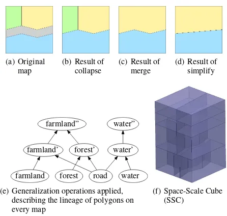
3.2 A step-wise sequence of generalization operations
Research into multi-representation databases has changed the no-tion that map generalizano-tion produces independent maps at dif-ferent scales — with derived and stored links between the objects with different levels of detail the maps are not completely inde-pendent (see e. g. Ellsiepen, 2007; Persson, 2004).
This notion of linking multiple representations is taken a step fur-ther by van Oosterom (2005) by introducing a step-wise general-ization process, where a merge operation is iteratively applied and a binary tree structure stores the result of those generaliza-tion operageneraliza-tions (into what is called the ‘tGAP face tree’). Storing the sequence of generalization steps leads to variable-scale data: at every step a reduction of the number of objects to be displayed on the map takes place.
Figures 4(a) – (d) show a sequence of generalization operations. First, a road object is split over its 3 neighbours, then the forest area is merged into neighbouring farmland and finally the bound-ary between farmland and water area is simplified. To cope with the results of the split operation we modify the original binary tree structure into a Directed Acyclic Graph (DAG) structure for storing the result. Figure 4(e) illustrates the resulting DAG.
3.3 The SSC as resulting 3D planar partition
(a) Original map
(b) Result of collapse
(c) Result of merge
(d) Result of simplify
water”
forest’ water’ farmland’
forest
farmland road water
farmland”
(e) Generalization operations applied, describing the lineage of polygons on every map
(f) Space-Scale Cube (SSC)
Figure 4: Illustration of generalization process and the resulting SSC.
Axiom 14. For a planar partition wherek = 3, the primitives P ∈ X have to be labeled as follows:
• p0
: two or more labels
• p1: two or more labels
• p2
: exactly two labels
• p3: exactly one label
Note that normally in a purely 3D topological setting an edge (p1
) should have three or more labels (and a node four or more). Furthermore, in our implementation setting, the labelling is based on the fact that we also want faces in the resulting SSC to be flat (similar to straight subsets in the 2D case):
Definition 12. Points in a face (p2
) are planar (in 3D following the equation:ax+by+cz+d= 0).
3.4 Incidence and adjacency revisited
The definitions and axioms describe what we term a valid space-scale cube in 3D. This cube captures the result of the general-ization process, but from this cube we can also determine what generalization operations were applied. The split, merge and sim-plify generalization operations introduce horizontal and vertical polygons (orthogonal to the space dimension) in the space-scale cube: Extruded boundaries between polygons in 2D (line seg-ments) become vertical (planar) polygons in 3D. As the polyhe-drons will have to have a boundary, a ‘roof’ primitive has to be put on top of a volume – these polygons define the end of the scale range for a polyhedron and will be parallel with the bottom plane of the space-scale cube (see Figure 4(f) and 6(a)). Note that for a single zone, there will be one polyhedron; e. g. the wa-ter zone extends from top to bottom in the SSC of Figure 4(f), but for orientation purpose some non-existing interior horizontal faces are depicted.
These parallel polygons define that two volumes are incident with each other in the scale dimension. This means that the top-most volume is the result of applying a generalization operation to the
other, lower volume. Thus the incidence relationship via hori-zontal polygons permits to derive what generalization operations were applied, i. e. this relationship captures the generalization process. Based on the incidence relationshipsdualityof the vol-umes can be defined – only in the vertical direction, the scale dimension, the duality really reflects the generalization process (‘scale neighbours’), while horizontally ‘normal’ space neigh-bours can be obtained.
4 OBTAINING VALID 2D MAPS FROM A SSC
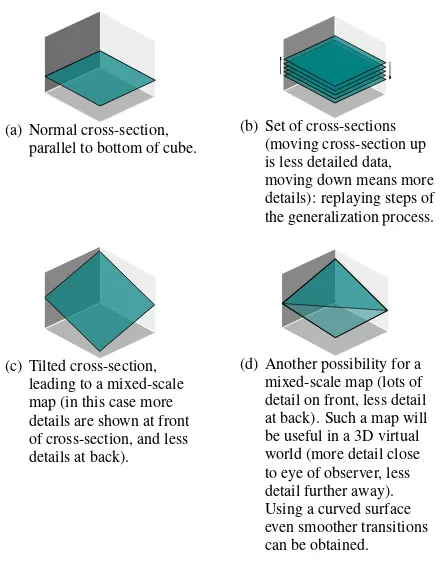
The axioms we have given in Section 2 and 3 define what we consider a valid 3D space-scale cube. We described the general-ization process as extrusion of a 2D planar partition into a third dimension (the level-of-detail-dimension) leading to a 3D parti-tion of space. Now we want the inverse of this process: deriving a 2D map from the 3D partition. Obtaining this map means to derive a cross-section of the 3D cube that is parallel with the bot-tom plane of the space-scale cube (Figure 5(a) illustrates taking such a slice).
Theorem 3. A derived 2D cross-section from a SSC will conform to the axioms for a valid 2D map.
Proof. The proof for horizontal slices is easy: at the bottom of the cube (finest detail, largest scale) the input was already a valid planar partition, every generalization operation makes sure that the next representation is again a valid planar partition, and in between only simple extrusion in the scale dimension takes place and then slicing is equal to the planar partition just below the slice plane.
For other, non-backfolding slicing surfaces the proof is less obvi-ous. In fact the result will be a ‘planar partition’ with potentially multi-part zones (which were not allowed according to our defi-nition of a valid planar partition).
When the cross-section is exactly colliding with horizontal prim-itives in the cube, it will be important to be careful when ‘slicing’ horizontally through the cube at a specific scale. Then the ques-tion arises, which of the 2 labels to display in the 2D map. The label to be shown would be the label of the top-most volume (as this then generates a consistent set of 2D maps, i. e. also at the bottom plane of the cube data will be shown).
Figure 5(b) shows another use of the cube: Obtain a sequence of cross-sections by moving the plane that defines a cross-section up or down in the cube. This way it is possible to re-play the steps of the generalization process showing how the map changes in the scale dimension. This can be beneficial for progressive transfer or smooth display. To efficiently encode differences between two cross-sections might however need different techniques (e. g. as in Haunert et al., 2009; Sester and Brenner, 2005), as data be-tween the first and second cross-section will be mostly similar.
5 CONCLUSION AND FUTURE WORK
This paper introduced the space-scale cube (SSC) as a theoretical framework guaranteeing valid data at any level of detail present in the cube. As representations are non-overlapping and the amount of detail is decreasing when going to the top of the cube, incon-sistencies in the derived 2D maps are also prevented. The space-scale cube thus provides provable consistent representations.
(a) Normal cross-section, parallel to bottom of cube.
(b) Set of cross-sections (moving cross-section up is less detailed data, moving down means more details): replaying steps of the generalization process.
(c) Tilted cross-section, leading to a mixed-scale map (in this case more details are shown at front of cross-section, and less details at back).
(d) Another possibility for a mixed-scale map (lots of detail on front, less detail at back). Such a map will be useful in a 3D virtual world (more detail close to eye of observer, less detail further away). Using a curved surface even smoother transitions can be obtained.
Figure 5: Possible cross-sections.
• How is the cube most efficiently represented in an imple-mentation, e. g. in a data structure with nodes, edges and faces, but without explicit vertical polygons (Meijers et al., 2009), or by indeed using a full topological 3D structure (c. f. Zlatanova et al., 2004, for alternatives)?
• Figure 5(c) and 5(d) show more possibilities for obtaining cross-sections using a tilted plane. This leads to a ‘mixed-scale’ map – i. e. a map with more detail in one part of the map than in the other parts of the map. This can be useful for 3D virtual worlds, where 2D data is projected into the 3D world, where close to the eye of the viewer more detail is required, compared to at a larger distance. A similar effect can be seen when a magnifying glass is placed over a 2D map (e. g. see Harrie et al., 2002) – in the SSC case this means that the cross-section is a bell-shaped plane.
One question is: Does such type cross-sections impose spe-cific requirements on the data structures for efficient retrieval of the resulting 2D map? Another question arises when such a mixed-scale map is derived, whether the axioms are not too strict. Intersecting with a non-horizontal slice plane can lead to multi-part polygons, which is disallowed by the cur-rent set of axioms (e. g. two patches of one polygonal area, one at one side of the map, one patch at the other side of the map).
• It would be possible to allow curves and curved surfaces as primitives inside the cube: This way a more continuous look and feel between cross-sections can be obtained leading to even ‘smoother’ visualizations or morphs (for progressive transfer).
• Instead of using just horizontal and vertical faces, defin-ing the prism parts of the polyhedra, it would als be pos-sible to use tilted faces. These would then be corresponding to a gradually changing representation (van Oosterom and Meijers, 2011). Our definition of a valid SSC further re-mains equal.
(a) Data inside the space-scale cube. Note that horizontal ‘roof’ polygons are left out and no simplification of boundaries was performed.
(b) Cross-sections of data from the space-scale cube at different levels of detail.
Figure 6: Example of a space-scale cube (looking from above into the cube) together with some derived cross-sections.
• How to extend the dimensionality of the cube into 4D (either increasing the dimension to 3D space, or adding a 1D time dimension) and even 5D (3D space, 1D time, 1D scale), as proposed by van Oosterom and Stoter (2010)?
ACKNOWLEDGEMENTS
The authors gratefully acknowledge the discussions with their colleague Hugo Ledoux, the constructive comments of Rod Thomp-son and the comments of 3 anonymous reviewers that helped to improve the paper.
References
Bader, M. and Weibel, R., 1997. Detecting and resolving size and proximity conflicts in the generalization of polygonal maps. In: Proceedings of the 18th International Cartographic Confer-ence. Stockholm, pp. 1525–1532.
Dyken, C., Dæhlen, M. and Sevaldrud, T., 2009. Simultaneous curve simplification. Journal of Geographical Systems 11(3), pp. 273–289.
Ellsiepen, M., 2007. Partial regeneralization and its requirements on data structure and generalization functions. In: H. Kremers (ed.), Lecture Notes in Information Sciences: 2nd ISGI 2007, CODATA, Berlin, pp. 72–84.
Erwig, M. and Schneider, M., 1997. Partition and conquer. In: S. Hirtle and A. Frank (eds), Spatial Information Theory A Theoretical Basis for GIS, Lecture Notes in Computer Science, Vol. 1329, Springer Berlin / Heidelberg, pp. 389–407.
H¨agerstrand, T., 1970. What about people in regional science? Papers in Regional Science 24(1), pp. 6–21.
Harrie, L., Sarjakoski, L. T. and Lehto, L., 2002. A variable-scale map for small-display cartography. International Archives of Photogrammetry Remote Sensing and Spatial Information Sci-ences 34(4), pp. 237–242.
Hoel, E. G., Menon, S. and Morehouse, S., 2003. Building a robust relational implementation of topology. In: T. Hadzi-lacos, Y. Manolopoulos, J. Roddick and Y. Theodoridis (eds), Advances in Spatial and Temporal Databases, Lecture Notes in Computer Science, Vol. 2570, Springer Berlin / Heidelberg, pp. 508–524.
L´evy, B. and Mallet, J.-L., 1999. Cellular modelling in arbitrary dimension using generalized maps. Technical report, Gocad Consortium.
Mackaness, W. A., Ruas, A. and Sarjakoski, L. T., 2007. Gen-eralisation of geographic information: cartographic modelling and applications. Elsevier Science Ltd.
Meijers, M., 2011. Simultaneous & topologically-safe line sim-plification for a variable-scale planar partition. In: S. Geert-man, W. Reinhardt and F. Toppen (eds), Advancing Geoin-formation Science for a Changing World, Lecture Notes in Geoinformation and Cartography, Springer Berlin Heidelberg, pp. 337–358.
Meijers, M., van Oosterom, P. and Quak, W., 2009. A storage and transfer efficient data structure for variable scale vector data. In: Advances in GIScience, Lecture Notes in Geoinformation and Cartography, Springer Berlin Heidelberg, pp. 345–367.
Persson, J., 2004. Streaming of compressed multi-resolution ge-ographic vector data. Geoinformatics, Sweden.
Sester, M. and Brenner, C., 2005. Continuous generalization for visualization on small mobile devices. In: P. Fisher (ed.), Developments in Spatial Data Handling, Springer-Verlag, pp. 355–368.
van Oosterom, P., 2005. Variable-scale topological data structures suitable for progressive data transfer: The GAP-face tree and GAP-edge forest. Cartography and Geographic Information Science 32, pp. 331–346.
van Oosterom, P. and Meijers, M., 2011. Towards a true vario-scale structure supporting smooth-zoom. In: Proceedings of 14th Workshop of the ICA commission on Generalisation and Multiple Representation, p. 17.
van Oosterom, P. and Stoter, J., 2010. 5D data modelling: full integration of 2D/3D space, time and scale dimensions. In: Proceedings of the 6th international conference on Geographic information science, GIScience’10, Springer-Verlag, Berlin, Heidelberg, pp. 310–324.
van Oosterom, P., Quak, W. and Tijssen, T., 2003. Polygons: the unstable foundation of spatial modeling. In: Proceed-ings ISPRS joint workshop on spatial, temporal and multi-dimensional data modelling and analysis, Quebec, Canada, p. 8.
van Oosterom, P., Stoter, J., Quak, W. and Zlatanova, S., 2002. The balance between geometry and topology. In: D. Richard-son and P. van Oosterom (eds), Advances in Spatial Data dling, 10th International Symposium on Spatial Data Han-dling, Springer-Verlag, Berlin, pp. 121–135.
Vermeij, M., van Oosterom, P., Quak, W. and Tijssen, T., 2003. Storing and using scale-less topological data efficiently in a client-server dbms environment. In: GeoComputation 2003, University of Southampton, Southampton, UK.