TOPOLOGY EXTRACTION USING DEPTH FIRST SEARCH ON VOXEL
REPRESENTATIONS OF TREE POINT CLOUDS
A. Schillinga, A. Schmidta, H.-G. Maasa, S. Wagnerb a
Technische Universität Dresden, Institute of Photogrammetry and Remote Sensing, 01062 Dresden, Germany b
Technische Universität Dresden, Institute of Silviculture and Forest Protection, 01735 Tharandt, Germany [email protected]
Commission V, WG 3
KEY WORDS: Forestry, Terrestrial Laser Scanning, Point Cloud, Forest Inventory, Topology Extraction
ABSTRACT:
The three-dimensional reconstruction of the vegetation structure is a requirement for the analysis of interaction between biosphere and atmosphere. Information about the 3D structure of plants enables the modeling of crucial processes, like water interception or absorption of light. Terrestrial laser scanners have proven to be a valuable tool to rapidly and accurately capture the geometry of plants as point clouds, which provide the foundation for analyzing their structure. Based on a very dense but unstructured, noisy point cloud, we have presented a method to extract the topology of a tree in form of a tree graph, demonstrated on a test set of single birches. In a first step we have applied a variation of the Circular Hough Transform to detect a set of 3D points, which represent the tree trunk. Subsequently, the point cloud is transformed onto a voxel space and filtered to a connected component representation of only the main object. In the second step, the residual voxels are interpreted as a connected graph and the Depth First Search algorithm is employed to retrieve the topology of the scanned tree.
1. INTRODUCTION
Terrestrial laser scanning (TLS) is an efficient method to capture accurate 3D geometry of real objects as point clouds. The point cloud representation of these 3D objects can be acquired rapidly and easily. The use of point clouds for forestry-related tasks is already rather appealing, because forestry measurements are often labor-intensive, limited to a few parameters and biased by the observing operator. The extraction of various forest inventory parameters has well advanced (Hopkinson et al., 2004; Maas et al., 2008), whereas capturing the complex tree structure is still a difficult task. Forests are described by their ecological characteristics, which are established by the actual structure of the individual trees. The distinctive forest structure governs processes such as water interception, absorption of light, and distribution of energy and precipitation. In order to gain a fundamental understanding of the interrelationships between physical characteristics of trees and environmental variables, detailed information on the structure of single trees is required. For that purpose, a detailed representation of the tree topology is an inevitable first step. We are focusing on single trees of a birch stock to identify segments like the trunk, branches, and twigs. These segments describe the topological composition of a tree, and will enable the determination of common parameters, for instance crown base height, crown diameter, tree height, and trunk diameter at breast height (DBH). Herein, a topology representation is not necessarily an actual skeleton of the tree, but rather an approximation of the spatial plant structure.
In this paper, we present an approach for extracting the topological structure of individual trees, which is applicable to unfiltered 3D TLS point clouds. The first step uses a variation of the Circular Hough Transform to find a set of 3D points distributed along the � axis and centered within the tree trunk.
Due to the high number of points, for instance, up to 10 million points per tree, the direct analysis of unstructured 3D point clouds is cumbersome. Therefore, the point cloud is transformed to a voxel space representation to reduce the total number of elements and to facilitate neighbor-related operations. Afterwards, voxels are subjected to a thresholding operation, and removed where appropriate. Subsequently, Connected Component Labeling is utilized to determine the number of components in the voxel space and the main component representing the tree is isolated. Because the voxel space can be interpreted as a graph, we employ a graph theory algorithm, called Depth First Search, to retrieve the tree topology.
The paper is organized as follows: Section 2 gives a brief overview of existing approaches to extract the topology of tree point clouds and ways to process 3D data. In Section 3 the study site is introduced and data capturing is illustrated. Our method is described in detail in Section 4. The following section discusses our approach and the resulting topology representation. Finally, the paper closes in Section 6 with the conclusion.
2. RELATED WORK
As terrestrial laser scanners become more powerful, also the handling of large point clouds proves to be increasingly demanding.
In (Xu et al., 2007) a nearest neighbor graph was created on the raw sparse point cloud. The shortest paths from each point to a predefined root point were retrieved by Dijkstra’s shortest path algorithm. Following, the amount of paths was condensed to a graph representing the main skeletal tree structure. A similar approach was presented in (Côté et al., 2009). In (Yan et al., 2009) an adjacency graph was built between clusters of points International Archives of the Photogrammetry, Remote Sensing and Spatial Information Sciences, Volume XXXVIII-5/W12, 2011
previously determined by repetitive application of k-means and fitting of minimum boundary cylinders. Though, the high point numbers in our test data make the usage of nearest neighbor graphs of raw point clouds infeasible.
Therefore, the application of grid- and voxel-based methods for analyzing TLS point clouds is widespread, because they facilitate handling of the point clouds. For instance, image processing methods can be applied, if the 3D TLS points are projected onto a discrete 2D grid. Accordingly, (Aschoff and Spiecker, 2004) have presented an approach to detect cross sections of trunks using the Circular Hough Transform. However, this method is not robust enough if the data contains a significant amount of noise. As suggested in (Schilling et al., 2011), using the 3D points directly for a Circular Hough Transform, exploiting the usually high number of 3D points on trunks, yields more distinct peaks in the accumulation array. Several publications have shown that utilizing a 3D grid simplifies working with huge point clouds: (Gorte and Winterhalder, 2004) have presented an approach based on Connected Component Labeling to segment a point cloud into contiguous branches of the tree. Connected Component Labeling is a 2D image processing technique that can be easily extended to 3D voxel space. In addition, (Gorte and Pfeifer, 2004) have analyzed the tree topology in the voxel space by also augmenting morphological operators to 3D voxel space. The procedure has been further improved and presented as Dijkstra Skeletonization in (Gorte, 2006) utilizing Dijkstra’s algorithm, as well. In (Bucksch and Appel van Wageningen, 2006) a graph-reduction approach for skeleton extraction has been introduced. An octree structure containing the tree point cloud is created and subjected to a set of rules. Though, loops are present in the resulting graph and need to be carefully removed again. The approach has been continuously enhanced and has been recently applied to imperfect point clouds (Bucksch et al., 2010). Furthermore, (Bienert et al., 2010) have employed a voxel space representation to perform a point distribution analysis of several voxels to identify structural elements.
Our approach consists of two parts: On the one hand, we apply a variation of the Circular Hough Transform to identify the trunk of the tree in a point cloud, using the raw 3D points directly. And on the other hand, we utilize a 3D voxel grid and propose the application of the Depth First Search algorithm as a novel way to retrieve the relevant skeletal tree structures efficiently.
3. STUDY SITE AND INSTRUMENTS
3.1 Study Site
For testing purposes, we used TLS point clouds, which were acquired in the scope of our research project. Our study site is a plain birch stock (Betula pendula)located approximately 15�� southwest of Dresden, Germany and under observation of the Chair of Silviculture of the TU Dresden for more than 40 years. The birch stock covers an area of about 1.3ℎ� (160�× 80�) and consists of more than 350 trees, which are about 55 years of age. Trunk diameters at breast height (DBH) were measured manually as a reference and range from 16.6�� to 34.4��; tree height varies from 27.8� up to 28.8�. The birch trees show an almost straight trunk until about half of the entire tree height.
3.2 Data Capturing
The birch stock was scanned using the Imager 5006i terrestrial laser scanner from Zoller+Fröhlich. The scanner employs a phase shifting technique and exhibits an average distance accuracy of 2.6�� at 25� on dark material (Zoller+Fröhlich, 2009). In order to ensure scan coverage as complete as possible of the entire study site, twelve ground positions have been established. Following, the twelve single scans were co-registered with the ZF-LaserControl software using 40 fixed targets mounted on selected trees. Scans were taken with an average angular scan resolution of 0.018° and limited to a maximum range of 37� afterwards. Because the point density decreases with distance, tree crowns are represented by significantly fewer points than trunks, and small structures cannot be resolved in detail. In addition, gaps occur in the scan data due to occlusions. The study site was scanned four times in 2010: in leafless condition, while leaves unfolding, with full leaves, and during leaf-fall.
The results, presented in this paper, were obtained using only the data sets of trees in leafless condition. A subset of 37 trees was selected and each tree was separated automatically, as in (Schilling et al., 2011). Thus, each tree point cloud encompasses a volume with a square base of 6�× 6� with the tree at its center. Points of a 3D point cloud originate from more than one scan positions, therefore the plant is represented from several sides. As can be seen in figure 1, point clouds contain a significant amount of noise.
a) b)
Figure 1. Input TLS point clouds with noise.
4. METHODS
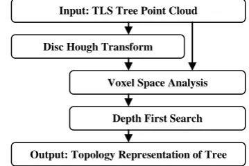
Our method processes unfiltered laser scanner points of single birch trees. The result is a set of polygonal lines approximating the tree topology. Extraction of the topology is fully automated with only a few parameters to be adjust beforehand. The general outline of our algorithm is summarized in figure 2. The following subsections discuss the separate phases in detail.
Figure 2. Processing scheme outline for topology extraction.
Input: TLS Tree Point Cloud
Disc Hough Transform
Voxel Space Analysis
Output: Topology Representation of Tree Depth First Search
4.1 Disc Hough Transform
A visual impression of the cross section of a point cloud can be obtained by projecting the 3D TLS points onto a discrete grid parallel to the ��-plane. Trunks appear as circle- or arc-like structures depending on scan coverage, which can be detected by the Circular Hough Transform, as detailed in (Sonka et al., 1998). Applying the Circular Hough Transform directly on the 3D points can yield more robust results if a lot of other structures caused by understory vegetation are present. Furthermore, as the radius of the trunk cannot be determined reliably in advance, a disc instead of a circle is employed for the accumulation step. We have termed this variation Disc Hough Transform. The use of a disc also overcomes the problem that a trunk cross section does not necessarily resemble a perfect circle.
In order to obtain 3D center points of assumed circular structures in the point cloud, the Disc Hough Transform is applied to the entire point cloud as follows: The input data is divided in slices of predefined thickness �� along the �-axis. Only the slices up to one third of the entire vertical extend of the data bounding box are considered. Furthermore, we restrict the slices to a circular area around the 2D slice center point. A Disc Hough Transform is conducted on each slice. For each slice, a copy of the accumulation array is binarized by a fraction of the maximal array value. Subsequently, the connected components in this array are identified. Reducing each component to the element with the highest array value in the accumulation array produces a set of 2D points per slice. A circle is fitted to a subset of 3D points for each of the determined 2D points in the current slice, as shown in (Schilling et al., 2011). 3D points located within a radius �� around the particular 2D point, considering their Euclidean distance in the ��-plane, are used for the circle fitting. The center point of each circle and its radius are stored per slice. In this way the entire input data is processed yielding a set of 3D points distributed in the ��-plane over a range of discrete �-Coordinates.
As a short segment of the trunk can be assumed to approximate a 3D line; RANSAC (Fishler and Boles, 1981) is then used to identify points contributing to a 3D line under a predefined error threshold. All points not contributing to the support set of the established trunk line are removed. If the remaining points do not exhibit spacing along the z-axis equal to ��, missing points are interpolated.
In brief, this phase produces a set � of 3D points with radius values. These points constitute a polygonal line that represents the skeleton line of the tree trunk in the point cloud data set. 4.2 Voxel Space Analysis
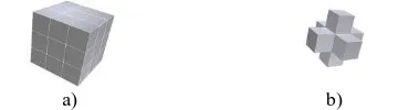
The tree point cloud is converted to a discrete voxel space representation, as illustrated in figure 3. Each voxel of the 3D matrix contains the number of 3D points it comprises. Voxels with a number of points less than a predefined threshold are cleared. A Connected Component Labeling, as described in (Shapiro and Stockmann, 2001), is applied on the 3D matrix. This operation considers the 26-adjacency of each voxel and labels them with the corresponding component index. Furthermore, voxels containing a 3D point of the set � are tagged as trunk. The index of the component containing these voxels is identified. Subsequently, all voxels are checked; if their component index does not match with the established index, they are cleared.
In summary, using the previously determined point set �, the connected components present within the voxel space are reduced to the particular one, which actually composes the tree. 4.3 Depth First Search
Depth First Search, as explained in (Russell and Norvig, 2010), is engaged to find a path from a particular start to a defined goal state. At each step, this general search algorithm evaluates its neighbors and moves to the neighbor which seems most appropriate. The most appropriate neighbor is usually determined by evaluation of a path-cost function �(�) considering all available neighbors. If the search cannot advance, because all neighbors have already been visited, the path is backtracked until an unexplored neighbor is encountered. If the current state is identified as a goal state, the algorithm finalizes. If no path can be found, the current path is backtracked to its start state.
a) b)
Figure 3. Voxel space representation of raw point cloud. In the following, the voxel space is interpreted as a single connected graph. Each non-empty voxel in the voxel space is considered a state and accordingly, the 26-adjacency of a voxel denotes its neighboring states.
Previously, a single connected component, representing the tree, within the voxel space was isolated. Clearly, there exists at least one path between a specific voxel to any other voxel within this component.
Because it might be more difficult to trace the branches beginning from the trunk, we are trying to trace paths starting at the branch endings. Moreover, it is a reasonable assumption that every branch is eventually connected to the trunk section of the tree. As voxels corresponding to the trunk have already been labeled accordingly, they are employed as goal states. However, the start states still need to be identified.
a) b)
Figure 4. Voxel with a) 26-adjacency and b) 6-adjacency. To identify voxels at branch endings their 6-adjacency, as depicted in figure 4b, is considered. All voxels above a predetermined height with less than three neighbors are regarded as potential branch ending voxels, as depicted in figure 5c and d. Each of them is employed as a start state for the International Archives of the Photogrammetry, Remote Sensing and Spatial Information Sciences, Volume XXXVIII-5/W12, 2011
search algorithm. Moreover, voxels composing a path from a start voxel to the goal are assigned an index identifying the particular path uniquely.
a) b)
Figure 5. a) and b) Isolated tree component with the set of branch ending voxels highlighted in green.
In our implementation of the Depth First Search, the path-cost function �(�) evaluates the Euclidean distance of the considered voxel to the closest goal state. Consequently, one of the neighbor voxels minimizes �(�); therefore, it is interpreted as the most appropriate choice for the next step. Here, the neighborhood comprises the entire 26-adjacency of the current voxel. The selection of the next voxel is performed in two stages. First, the neighbors are inspected whether a path already passes through any of them. In this case, those neighbors are preferred and the one minimizing �(�) is selected. Hence, if the current path encounters an already established path, the search is terminated and paths are linked together. Second, if no path passes the vicinity of the current voxel, the path-cost function �(�) is evaluated for all of the neighboring voxels accordingly.
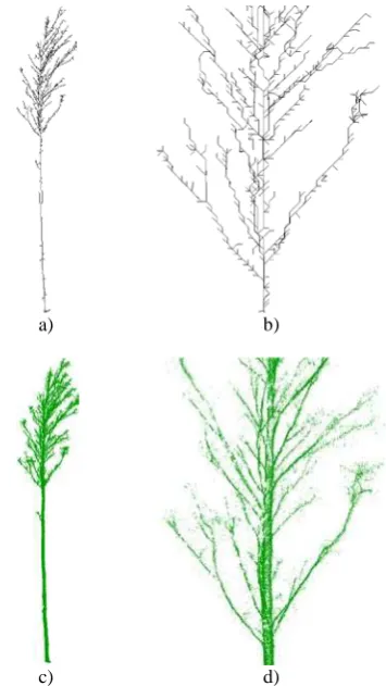
A Depth First Search is performed for each of the potential branch ending voxels. In each application of the search algorithm a different path through the voxel component is retrieved. The total amount of paths constitutes the tree topology representation, as illustrated in figure 6a and b. 4.4 Topology Representation
The output of our method is a tree in a graph theoretical sense resembling the trunk and branching structure of the scanned physical tree, as shown in figure 6a and b. Nodes in the tree graph are 3D center points of voxel passed by a search path. Each node is linked to its precursor and one or more successors, in case it is a branching node. Furthermore, the tree graph does not contain loops due to two constraints of the Depth First Search: Neighbor voxel are only considered as a valid next step if they have not already been visited. An exception is made, if a path crosses through the neighbor voxel and the current search could thus be terminated in the next step. Similarly, start voxel are only considered for a search, if they are unvisited and do not already belong to a previously found path.
5. RESULTS AND DISCUSSION
In figure 3, 5 and 6 results of the different stages of our method are demonstrated on typical data sets. Hence, the function of our method is twofold. On the one hand, it can be applied as a filter to the tree point cloud. If all points that are further away from the closest topology segment than a predefined threshold are removed, the resulting point cloud comprises almost exclusively 3D points, which are actually located on the tree surface, as depicted in figure 6c and d. On the other hand, it is a
way to swiftly compute an approximation of the tree topology. In the following subsections the parts of our method are examined separately.
a) b)
c) d)
Figure 6. a) and b) Tree topology representation. c) and d) The filtered tree point cloud. 5.1 Disc Hough Transform
Both the Disc Hough Transform and its application on each height interval account for the robustness of this part of our method.
Because of the high scan coverage in our data sets, the trunks are represented by a large number of points. This circumstance is exploited by the Disc Hough Transform as it generates distinct peaks at trunk centers in the accumulation array. In our tests, the threshold value for array binarization was set to one sixth of the largest value of the array. Therefore, the threshold value depends on the considered height slice. Of course, if trunks are weakly represented, they will hardly be recognized if denser understory vegetation is present as well. The threshold value was determined empirically and performs well on our data. However, a more sophisticated approach to identify the important peaks in the accumulation array would be preferable. Ideally, the consecutive analysis of all stacked slices produces a trunk point at each height interval. Even if scan points at the trunk surface are lacking in some heights, because of occlusions from other vegetation, usually a sufficiently large number of points is found. In fact, only the resulting ample amount of trunk points allows the application of RANSAC to recover a trunk line in the set of points. The MATLAB implementation of RANSAC by (Kovesi, 2011) was employed in our tests, which finds a trunk line with a sufficient large set of supporting points usually within a few iterations. Trunks could be easily missed if International Archives of the Photogrammetry, Remote Sensing and Spatial Information Sciences, Volume XXXVIII-5/W12, 2011
only a few slices would be examined. Moreover, it would be considerably more problematic to identify the trunk points correctly.
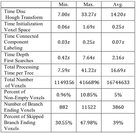
Currently, the MATLAB implementation of the Disc Hough Transform is the slowest part of our method, as can be concluded from the averaged performance values on our test data in table 7.
Table 7. Performance values of the method on the previously selected 37 tree data sets.
5.2 Voxel Space Analysis
For efficiency reasons, all operations in the voxel space were implemented in C++. In case of a point cloud containing solely a single tree, only a few percent of the entire voxel grid actually do contain 3D points. Hence, if the voxel cell size does not fall below ca. 5��, the grid can be easily kept in main memory as a one dimensional array, which also provides fast element access. Furthermore, the Connected Component Labeling employs a union-find data structure with path compression, as detailed in (Shapiro and Stockmann, 2001), for memory- and time-efficient labeling of the voxel grid elements.
The cell size of the voxel grid need not be equal to the cell size of the accumulation array used by the Disc Hough Transform. However, it facilitates the evaluation of the results and an equally small value for both cell sizes is feasible.
Another important parameter of the voxel space analysis is the required minimum number of 3D points per voxel, which is used for initial filtering of the voxel grid. In fact, both parameters are interdependent: The smaller a voxel is, the fewer points it may contain. This relation governs how close the connected components approximate the natural shape of the tree. Because of occlusions and depending on the parameters, branch parts can appear as separate components. Whereas, crowns of nearby trees might also be connected to the targeted tree component if they are too close together. Since we do not analyze the particular component shape in the voxel grid, we cannot avoid such configurations at the moment. Though, linking components which are close to each other might be easier than classifying separated components directly as tree parts. In addition, interconnected crowns may be detectable in
the topology representation, as suggested by our preliminary tests. We used a cell size of 10�� and 10 as the required minimum number of points per voxel.
5.3 Depth First Search
On the voxel grid, Depth First Search was implemented in C++ without any particular optimization. As can be seen in table 7, the search algorithm is quite fast on this data
Using our definition, as mentioned in Section 4.3, the number of start voxel is between several hundred and a few thousand. The large number of path searches does not induce significant time overhead for two reasons: First, a lot of searches result in very short paths to the next path crossing nearby; and second, because a voxel loses its status as a start voxel if it is passed by a path starting elsewhere. Therefore, a bit less than half of all potential start voxel are usually skipped by the search algorithm. However, voxels which are not explicit branch ending voxels, but rather border voxels of branches result in short paths, which are not a reliable representation of the actual plant topology. The length of the shortest possible path segment equals the voxel cell size.
The performance of Depth First Search depends on the path-cost function �(�) and the function determining the next possible states to move to. In our method, the Euclidean distance to the trunk is minimized, constraining the search to advance downward if possible. Regarding the tall birch trees in our test data sets, this behavior is suitable. Nevertheless, it will also find a path, if the branches do not grow monotonously upward, because the next step can advance to any valid state of the 26-adjacency of the current state. The search will initially explore any path that leads downward, until advancing to above neighbors remains the only alternative to backtracking the path, which is the very last option. In this case, the time necessary to find a path might be a bit longer, but we did not experience any significant impact on the runtimes.
5.4 Topology Representation
Clearly, the resulting topology representation is not a skeleton, because the tree segments are not centered within their surrounding 3D points. Furthermore, the path finding process is deterministic only insofar as the order of start voxel, which are consecutively processed by the search algorithm, stays the same. We observed that it is beneficial for our tall birch trees if the set of start voxel is sorted by their � coordinate in decreasing order previous to the path finding process. In this way, long paths from the very top of branches to the trunk are found first. Then, the larger part of the other paths is usually quite short and linked to one of the few longer paths. As can be seen in figure 6a and b, the resulting tree graph is rather unrefined and needs further improvement. In some cases, a branch of the tree consists of a series of shorter paths that would have to be joined to a single longer segment. Afterwards, a filtering operation to remove short paths would be feasible to reduce the graph to the significant main structure.
These enhancements of the topology representation would allow the automatic extraction of several important forest inventory parameters. During the Disc Hough Transformation, as already mentioned in Section 4.1, a circle is fitted to a selected set of 3D points around each determined peak. Hence, for each thusly detected trunk point, the radius of the trunk at this height is already available. Though, for the correct determination of the diameter at breast height, information International Archives of the Photogrammetry, Remote Sensing and Spatial Information Sciences, Volume XXXVIII-5/W12, 2011
about the ground height is necessary. If the tree is represented well in the scan, the Disc Hough Transform can detect points down to the lowest height interval containing a part of the tree trunk. In this case, the lowest detected point can be assumed as the trunk foot point and used to determine the diameter at breast height relative to that. Otherwise, a digital terrain model has to be generated from the point cloud, for instance as in (Bienert et al., 2006), to compute the breast height exactly.
The tree height cannot be inferred directly from the topology representation, yet. Because of weak scan coverage of the higher, finer branches in the tree crown, they are usually cleared by the initial filtering step and not part of the component in the voxel space. Therefore, the topology representation might not rise as tall as the real tree. But, with a suitable offset to the height extent of the representation, a rough estimate of the actual tree height would be possible. In addition, the crown diameter might be assessed similarly.
However, the lower branches of the tree are normally recovered with sufficient accuracy. Therefore, the automatic detection of the crown base height from our topology representation would be feasible. At present, the topology representation has been evaluated solely by visual inspection. Though, we are striving to come up with a method for an objective evaluation.
6. CONCLUSION
In this paper, we have presented a method to generate a topology representation in form of a tree graph from point clouds of single trees captured by a terrestrial laser scanner. Our strategy involves a variation of the Circular Hough Transform, to detect arc- or circle-like 3D point subsets and an analysis of the connected component identifying the tree in the voxel space. Furthermore, the Depth First Search algorithm is employed to find paths from the branch ending voxels to the trunk. The resulting tree graph consists of smaller linked paths and outlines the principal topology of the scanned tree. Our method can, for instance, be applied to filter a noisy point cloud: If points are not close enough to the topology representation, they can be removed. An advantage of the proposed method is its simplicity and efficiency that allows for fast computation of the topology representation, which is, of course, our main objective.
At present, the resulting tree graph is only an approximation of the tree topology. With further enhancements, it could provide a crucial intermediary step to enable an entirely automatic assessment of important forest inventory parameters, which we will investigate in the future.
ACKNOWLEDGMENT
The work presented here was funded by DFG (Deutsche Forschungsgemeinschaft). The Zoller+Fröhlich scanner was kindly provided by the Institute for Traffic Planning and Road Traffic (Prof. Dr. Lippold, TU Dresden).
REFERENCES
Aschoff, T., and Spiecker, H., 2004. Algorithms for the automatic detection of trees in laser scanner data. In: International Archives of Photogrammetry, Remote Sensing and Spatial Information Sciences, Vol. 36, Part 8/W2, pp. 71-75.
Bienert, A., Scheller, S., Keane, E., Mullooly, G., and Mohan, F., 2006. Application of Terrestrial Laser Scanners for the Determination of Forest Inventory Parameters. In: International Archives of Photogrammetry, Remote Sensing and Spatial Information Sciences, Vol. 36, Part 5.
Bienert, A., Queck, R., Schmidt, A., Bernhofer, C., and Maas, H.-G., 2010. Voxel space analysis of terrestrial laser scans in forest for wind field modelling. In: International Archives of Photogrammetry, Remote Sensing and Spatial Information Sciences, Vol. 38, Part 5, pp. 92-97.
Bucksch, A., and Appel van Wageningen, H., 2006. Skeletonization and segmentation of point clouds using octrees and graph theory. In: Proceedings of Commission V Symposium, Image Engineering and Vision Metrology, Dresden, Germany, pp. 1-6.
Bucksch, A., Lindenbergh, R., and Menenti, M., 2010. SkelTre - Robust skeleton extraction from imperfect point clouds. Visual Computer, 26, pp. 1283-1300.
Côté, J.-F., Widlowski, J.-L., Fournier, R.A., and Verstraete, M.M., 2009. The structural and radiative consistency of thee-dimensional tree reconstructions from terrestrial lidar. Remote Sensing of Environment, 113, pp. 1067-1081.
Fishler, M.A., and Boles, R.C., 1981. Random sample concensus: A paradigm for model fitting with applications to image analysis and automated cartography. Comm. Assoc. Comp, Mach., 26, pp. 381-395.
Gorte, B., 2006. Skeletonization of Laser-Scanned Trees in the 3D Raster Domain. Innovations in 3D Geo Information Systems. Lecture Notes in Geoinformation and Cartography. Springer, Berlin Heidelberg, pp. 371-380.
Gorte, B., and Pfeifer, N., 2004. Structuring Laser-scanned trees using 3D mathematical morphology. In: Proceedings of the XXth ISPRS Congress: Geo-Imagery Bridging Continents, Turkey, Istanbul, pp. 929-933.
Gorte, B., and Winterhalder, D., 2004. Reconstruction of laser-scanned trees using filter operations in the 3D raster domain. In: International Archives of Photogrammetry, Remote Sensing and Spatial Information Sciences, Vol. 36, pp. 39-44.
Hopkinson, C., Chasmer, L., Young-Pow, C., and Treitz, P., 2004. Assessing forest metrics with a ground-based scanning lidar. In: Canadian Journal for Forest Research, Part 34, pp. 573-583.
Kovesi, P., 2011. MATLAB and Octave Functions for Computer Vision and Image Processing.
http://www.csse.uwa.edu.au/~pk/research/matlabfns/ (13. April.2011).
Maas, H.-G., Bienert, A., Scheller, S., and Keane, E., 2008. Automatic forest inventory parameter determination from terrestrial laserscanner data. International Journal of Remote Sensing, 29, pp. 1579-1593.
Russell, S., and Norvig, P., 2010. Artifical Intelligence. 3rd ed., Prentice Hall, pp. 87-89.
Schilling, A., Schmidt, A., and Maas, H.-G., 2011. Automatic Tree Detection and Diameter Estimation in Terrestrial Laser Scanner Point Clouds. In: Proceedings of the 16th Computer Vision Winter Workshop. Mitterberg, Austria, pp. 75-83.
Shapiro, L.G., and Stockmann, G.C., 2001. Computer Vision. Prentice Hall, pp. 69-75.
Sonka, M., Hlavac, V., and Boyle, R., 1998. Image processing, analysis, and machine vision. 2nd ed., PWS Publishing, pp. 163-173.
Xu, H., Gossett, N., and Chen, B., 2007. Knowledge and heuristic-Based Modeling of Laser-Scanned Trees. ACM Transactions on Graphics, 26.
Yan, D.-M., Wintz, J., Mourrain, B., Wang, W., Boudon, F., and Godin, C., 2009. Efficient and robust tree model reconstruction from laser scanned data points. In: Proceedings of the 11th IEEE International conference on Computer-Aided Design and Computer Graphics, pp. 572-576.
Zoller+Fröhlich, 2009, Broschure Imager 5006i.