KEY WORDS:Palm Trees, Detection, Circular autocorrelation of polar shape matrix, CAPS, Shape feature, SVM
ABSTRACT:
Palm trees play an important role as they are widely used in a variety of products including oil and bio-fuel. Increasing demand and growing cultivation have created a necessity in planned farming and the monitoring different aspects like inventory keeping, health, size etc. The large cultivation regions of palm trees motivate the use of remote sensing to produce such data. This study proposes an object detection methodology on the aerial images, using shape feature for detecting and counting palm trees, which can support an inventory. The study uses circular autocorrelation of the polar shape matrix representation of an image, as the shape feature, and the linear support vector machine to standardize and reduce dimensions of the feature. Finally, the study uses local maximum detection algorithm on the spatial distribution of standardized feature to detect palm trees. The method was applied to 8 images chosen from different tough scenarios and it performed on average with an accuracy of 84% and 76.1%, despite being subjected to different challenging conditions in the chosen test images.
1. INTRODUCTION
Remote sensing is widely used in different sectors of vegeta-tion monitoring like forestry, agriculture, biophysical studies etc. It includes identifying, classifying, localizing, measuring sizes, heights, carbon yields etc., which describe the characteristics and the socio-economic and environmental importance of different vegetation and ease the associated institutions in planning and monitoring.
In agriculture, palm tree cultivation is one of the big sectors with a huge market value. Palm trees are used to produce a variety of products like vegetable oil, bio-fuel, papers, furniture, decora-tions, fodder for cattle etc. It also has to be mentioned that palm oil is the most widely used vegetable oil in the world. In 2011, palm tree plantation produced over 53 million metric tons of palm oil in 16 million hectares land. The global production of palm oil is increasing every year along with its demand. According to forecast, in Indonesia and Malaysia alone which represent over 90% of palm oil produced globally, the production will increase by 30% by the year 2020 (Economy et al., 2014).
In order to meet this demand, it is necessary to plan well during cultivation and to monitor different aspects of trees like proper in-ventory, health, size, heights etc., at different stages of their life. As palm tree cultivation zones are huge and difficult to be moni-tored visually on ground, remote sensing can play a vital role in delivering those data and analysis, cost and labor efficiently from the satellite or aerial images. Therefore, this study investigates on one aspect, more specifically localizing and counting palm trees for creating their inventory, as an initial step towards the multi-faceted monitoring.
A few studies in this direction have already been published. Ju-soff and Pathan (2009) used the hyperspectral image to map palm trees. The study implemented the linear spectral mixture analysis to discover contributions of different materials on hyperspectral pixel vectors, then used the mixed-to-pure converter that assigns
those vectors to signatures and the minimum distance based for-mula to detect palm trees. Unfortunately, the results were not discussed in the publication. Hence, the performance of this ap-proach is difficult to compare. In general, the hyperspectral imag-ing shows a coarser geometrical resolution than three-channel im-ages and requires more expensive equipment.
Malek et al. (2014) have formulated a very well described frame-work for 2D image processing and analysis, in order to automati-cally detect the palm trees in images captured with unmanned air vehicle (UAV). The method uses shift invariant feature transform (SIFT) as a feature and extreme learning machine (ELM) and level setting for classification and grouping respectively. It is fol-lowed by the texture analysis of palm trees with local binary pat-terns (LBP). The performance of the framework is in general ad-mirably above 90%. In the method proposed by Shrestasathiern and Rakwatin (2014), they compute semi-variograms from the rank transformed vegetation index and use non-maximal suppres-sion on them to detect the peaks that correspond to the locations of the palm trees. The normalized difference index (NDI), which is the normalized ratio between green and red spectral bands of the image, is used as vegetation index, in order to make the pro-cess usable even for RGB images. And rank transformation is used for removal of blurred object borders to increase the dis-continuity between palm tree and background intensities. The performance of the method is stated as 90%.
(a)
(b)
Figure 1: (a) Model of a star-shaped object. (b) Polar shape matrix representation of the model
those drawbacks. As an extra feature for above algorithms, shape features could strengthen the algorithm’s potential.
This paper proposes a generic shape feature, the circular auto-correlation of the polar shape matrix representation of the image and uses this feature to detect palm trees. The study uses lin-ear support vector machine (SVM) to reduce the dimensions and standardize the CAPS and local maximum detection algorithm to detect the centers of palm trees canopy.
2. METHODOLOGY
The proposed method uses a sliding window approach for fea-ture extraction. A window of fixed size translates over the entire image, where algorithm derives CAPS for each window, reduces its dimension to single scalar value (standardized feature) and as-signs the standardized feature to the image pixel at the center of the window. It results in a spatial distribution of the standardized feature called feature map. The feature map consists of peaks on the palm trees with local maximum value at the center. Therefore, a local maximum detection algorithm is used on the feature map to detect palm trees. The local maximum detection algorithm re-sults in object map, which is the spatial distribution of the centers of the palm trees over the image. The detailed description of the method is presented in following subsections.
2.1 Palm Tree Model
In orthophotos, the palm tree canopies resemble star-shaped ob-jects with varying numbers of petals. Each palm tree grows 20-25 leaves every year (Food & Agriculture Organization of United Nation, 1977), but we found through the observation of multiple palm trees that the number of distinguishable leaves is limited to 8-12 petals due to their overlapping nature. In this study, a model of the star-shaped object, as in Figure 1, is used as the ba-sis to understand the characteristics of the star-shaped object and to develop a hypothesis about generic shape feature. The model consists of 10 leaves and the brightness of the object increases radially inward, with the highest value at the center. The back-ground is completely ignored for the analysis, which is not the case in the real-world scenario.
Star-shaped objects are radially symmetric and each pair of con-secutive leaves have a constant angular difference. Sampling the object along the circumference of a circle that is sufficiently large enough to include leaves results in a periodic curve with a period equivalent to the number of petals. Sampling along a number of such concentric circles centered at the center of object results to a two-dimensional matrix, with one axis being the angle and other being the radius, called polar shape matrix (Taza and Suen, 1989). The polar model shape matrix of the star-shaped object produces
a distinct triangular waveform like structure, as shown in Figure 1b.
The circular shift along the angular axis of the polar shape matrix results in the repetition of the same image when the shift is equiv-alent to the angular difference between leaves. The similarity de-creases until it reaches the least when the shift is half the angular difference between leaves, and gradually increases to maximum on the other half. This scenario repeats periodically with the pe-riod equivalent to the number of leaves. In order to measure the similarity between original polar shape matrix and the circularly shifted version of it, correlation coefficients can opt.
2.2 Circular Autocorrelation of Polar Model Shape Matrix Circular autocorrelation of polar model shape matrix (CAPS) is the generic shape feature proposed in the study, which is the cor-relation of a polar shape matrix representation of the object with a circularly shifted version of itself along the angular axis (circu-lar autocorrelation along angle). CAPS is a periodic curve with the number of peaks equivalent to the numbers of leaves, in the case of the ideal star-shaped object. A vector representing CAPS curve acts as the generic shape feature for detection method.
The polar shape matrix representation of the image is calculated by sampling image along the circumference of different concen-tric circles in a constant angular interval. Considering angular and radial sampling intervals αand β, the polar shape matrix representation of the image is given by;
Zrθ=Zxy(xm+r∗(cos(θ))T, ym+r∗(sin(θ))T) (1)
whereZxyis the image normalized to zero mean and unit stan-dard deviation,θ= (0, α,2∗α, ...,360−α)T,r=
(0, β,2∗β, ...., dmin/2)T anddminis the side with minimum diameter required to include object andxmandymare the coor-dinates of the center of the object.
Circular shifting is achieved by shifting the final entry to the first position while shifting all other entries to the next position. Cir-cularly shifting along the angle and calculating correlation for each shift is highly inefficient. Therefore, an efficient algorithm based on Wiener-Khinchin theorem is proposed as in Equation 2, which computes the autocorrelation through inverse Fourier transform of the product of Fourier transform of polar shape ma-trix and its conjugate.
ACR=real(F−1
{F{Zrθ} . F∗{Zrθ}}) (2)
whereF is the Fourier Transform.
autocor-relation values at different angular and radial shifts. The auto-correlation values are dependent on the gray level distribution in the image, more specifically, the overall lighting condition. The well-lit image that has larger pixel values has larger tion values and vice-versa. Therefore, the range of autocorrela-tion values varies between images. To overcome this variaautocorrela-tion, the autocorrelation values are normalized to Pearson autocorre-lation coefficients, where the values range from -1 to 1, -1 being inversely and +1 being positively correlated. The normalization method is mathematically described by the following equation:
R=ACR−N µ
2
Z
N σ2
Z
(3)
whereN is the total number of samples or elements in polar shape matrix.µZandσZare mean and standard deviation of polar
shape matrix.
The proposed feature considers the autocorrelation value along the angular shift only. Therefore, only the values at zero radial shift are extracted from the normalized Wiener-Khinchin product of polar shape matrix, as shown in Figure 3. Additionally, the autocorrelation function is symmetric in nature, hence only half of this vector i.e 360
2∗α number of elements is enough to describe the object and is used as the feature vector.
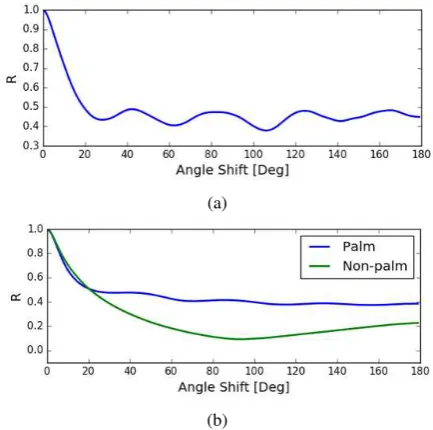
Figure 3: Circular autocorrelation of polar shape matrix.
CAPS has maximum values at zero angular shift, but for the ro-tationally periodic object it has multiple maximum values. The CAPS of the rotationally periodic object is itself periodic with the half the period. Circular autocorrelation, by nature, is not affected by the shift. In the case of CAPS, the shifting operation is carried out along the angular axis, therefore, CAPS is not affected by ro-tation. CAPS is invariant to overall illumination change, however slightly variant to the change in the direction of the source of light and variation of light within the object.
2.3 Feature Dimensionality Reduction and Standardization
CAPS is a vector with multiple elements, a total of 360 2∗α in num-ber. The collective influence of all these elements plays a decisive role in discriminating the objects. But, the higher dimensionality of the CAPS offer complexities in processing the features to de-tect objects. We propose the use of any standard machine learning methods, in our case linear SVM, as a transformation measure to reduce the dimension of this vector. SVM is a standard tool for
the training examples. The input feature vector formulates a com-plex multidimensional space where SVM determines the best de-cision boundary between positive and negative training examples (Figure 4) and the function to calculate the distance of examples from decision boundary in the same space. This reduces the n-D feature space to the 1-n-D scalar quantity with higher values for higher object likelihood.
Figure 4: Support Vector Machine: Red boundary is the hy-perplane generated by SVM by maximizing the margin with two blue hyperplanes, also called support vectors.
SVM uses the convex optimization method to determined the de-cision boundary/hyperplane in multidimensional feature space. If a training dataset{(xi, yi)}ni=1wherexi, also calledexample, is theith
vector andyiis the label associated withxiis used to train SVM. The decision boundary/hyperplane is identified by solving the following primal optimization problem.
min
W,b k
Wk2/2 +C n
X
i=1
ξi (4)
subject to,
yi.(WTxi+b)≥1−ξi i= 1, ..., n (5)
whereWT represents weight vector,ban explicit bias parame-ter (Liu et al., 2012, Ben-Hur and Weston, 2010, Bishop, 2006). The hyperplane or decision boundary is defined by the vectorx
such that the value of the discriminant function is zero. The mar-gin error0 ≤ ξi ≤ 1allows the samples to be in the margin or misclassified. The constantC >0is a regularization param-eter. Minimization of Equation 4 gives the unique solution of hyperplane which serves as the linear decision boundary for two classes.
The SVM is a discriminative model, hence, it provides the deci-sion rather than posterior probabilities. Decideci-sion function is given by
sgn(f(x) =WTx+b) (6)
Figure 5:f(x)of test samples from decision boundary
confidence measure. The decision function outputs the class label which input vectorxbelongs to (Chang and Lin, 2011).
Generally, the trained classifier is used with a sliding window de-tector which visits every pixel, calculates feature for the window around that pixel and, based on this feature, decides whether the pixel is object or non-object i.e. it labels the pixel directly us-ing the decision function in Equation 6. Usually, this approach generates many detections in the proximity of and within objects, which need to be post-processed.
In this study, instead of the decision on labels of windows, actual values of thef(x)are computed, as shown in Figure 5. Hence, linear SVM is rather used as the feature space transformation function, which reduces the dimensionality of the feature space from n-dimensional space to one-dimensional space, with the de-cision boundary as the referenceRn
=>R.
2.4 Local Maximum Detection
Feature map is a spatial distribution of standardized features over the image, with positive peaks on the palm trees with a local max-imum at the center of the palm trees, given that the features used for training are extracted from the blocks with the central pixel at the center of palm trees. The spatial extent of peaks depends on the size of objects.
To detect the locations of the objects, a local maximum detec-tion algorithm is proposed which, in the context of this study, is the sliding window algorithm where a window of definite size (footprint) translates over the entire image and calculates the lo-cal maximum by comparing the central pixel value to all other pixels values within the footprint. In the presence of non-palm objects, there could be local maximum detections on non-objects as well, hence, a threshold in the value off(x)is introduced such that only local maximum value exceeding this threshold is con-sidered as palm-trees. Figure 6 shows the visual demonstration of the algorithm, where the highest peak within a footprint that is above the feature-value threshold is detected. The result of detec-tion might vary a lot for different footprint sizes and thresholds. Therefore, an appropriate size of the footprint,Parameter Aand the threshold,Parameter Bhave to be chosen by evaluating accu-racies for different footprints and thresholds. The final result of this process is a distribution of the object’s center locations over the entire image: object map.
2.5 Accuracy Assessment and Optimization
2.5.1 Accuracy Assessment The detection results are evalu-ated by comparing them with the ground truths. Ground truths
Figure 6: Local maximum detection
are generated by manual selection of all object locations in the images. The precision-recall or users-producers accuracy, total accuracy and RMS localization error are computed for accuracy assessment.
The precision-recall and total accuracy is calculated from ratios of positives and negatives. For determining true and false posi-tives and negaposi-tives, the user should provide the maximum permis-sible localization error (δ) i.e. permissible deviation of location in ground truth and detection.
Precision or user’s accuracy is defined as the proportion of de-tected objects that are correct in reality, given by Equation 7. Re-call or producer’s accuracy is defined as the proportion of objects detected (Equation 8) (Powers, 2011). Total accuracy is calcu-lated as the average of both user and producer accuracy.
AccU= T P
T P+F P (7)
AccP = T P
T P+F N (8)
Acctot=P recision+Recall
2 (9)
2.5.2 Parameter Optimization As discussed before, the lo-cal maximum detection algorithm uses two parameters: footprint size and the feature-value threshold. The detection results are af-fected by the choice of values for those parameters and it is diffi-cult to choose those parameters, as they can vary between scenes and depend on size and shape of the palm trees. Therefore, an au-tomatic approach to determine those parameters is proposed here. But, it requires an image of small region per scene with ground truths.
In this approach, the local maximum detection algorithm is ap-plied to these images, choosing a set of varying footprint sizes and the feature-value thresholds. The precision, recall, and total accuracies are calculated for each of the detection results and the parameters corresponding to the highest accuracy are chosen as the final optimized parameters for the scene, where that image is taken from, as mathematically expressed in Equation 10.
A, B|max
A,B Acctot
(10)
3. STUDY AREA AND DATA 3.1 Study Area
Our study areas comprise of the oil-palm tree plantation regions in Malaysia, Thailand and Indonesia. Indonesia and Malaysia are the two biggest exporters of oil-palm tree products, which contribute to more than 90% of worldwide export (Colchester, 2011). The study data are aerial images captured at four planta-tion region in the stated countries, with Trimble UX5 unmanned aircraft system (UAS). Ground sampling distance of data range from 3.2 to 10 cm and consist of three spectral channels which include near-infrared, red and green in two of them and red, green and blue in others. The spectral combination of the image does not play a significant role in our study, hence, it is ignored and the only green channel is used for all the experiments. All of the data are orthorectified and reprojected to the Universal Trans-verse Mercator (UTM) projection system with World Geodetic System 1984 (WGS84) as an ellipsoid of the reference.
3.2 Training Data, Test Data and Ground Truth
Figure 7: Few examples of positive samples (Palm) of training data in the red channel.
The data chosen for training and test are resampled to approxi-mately 5 cm to avoid different sizes of training and test images. Through the observation in a significant amount of fully grown tree canopies, we found out that the canopies of the fully grown palm trees are enclosed by the window size of 201x201 pixels (10mx10m). Therefore, the sizes of training data and the window in feature extraction are chosen to be 201x201 pixels.
Training data are selected randomly from only one test site in Thailand. Training data consist of 644 samples of palm trees and 597 samples of non-palm objects, which include non-palm trees, cars, buildings, backgrounds etc. Few samples of the training data are shown in Figure 7. The leaves and their sizes varies between the images. In some cases, the leaves overlap and the canopies tend to be a circular object. On most of the training data, there are interferences of nearby trees or other objects.
Medium, Small
Img 04 Medium Low Yes Large
Img 05 Low Low No Medium
Img 06 High High No Large
Img 07 High High Yes Large
Img 08 Very Low Low No Large,
Medium, Small
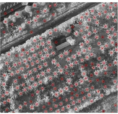
(a) (b)
Figure 8: (a) Test Image 07 (b) Test Image 08
Test images are selected from all the data, considering different challenges. In total, eight test images covering 4000x4000 pixels are selected. General characteristics of the test images selected are shown in Table 1. Within and between test images, the exis-tence of different cultivation densities, different levels of contrast between object and background, different sizes of trees, artificial objects etc. pose ample challenges for the algorithm to perform. Figure 8 demonstrates two of the test images used in the study. Figure 8a have a high cultivation density of palm trees that have a high resemblance to the star shape. The object-background con-trast is high and there are artificial objects like houses present. On the other hand, Figure 8b consists of palm trees, which have more circular shape with a low cultivation density. There exist palm trees of different sizes and the object-background contrast is very low. It is difficult, even for human eyes, to distinguish between the palm trees and the background. The ground truths required for accessing the accuracy of the study is prepared by manually selecting the palm tree centers in the test images.
4. IMPLEMENTATION AND RESULTS
of each element of CAPS for all palm and non-palm training ex-amples, where the average value of each element for palm trees are above 0.4 and most of the elements are demonstratively higher than that for non-palm training examples.
(a)
(b)
Figure 9: (a) CAPS of a palm sample (b) Average CAPS of all palm and non-palm training samples
The window of size 201x201px is translated over the test images to generate feature maps. The window is shifted along rows and columns at the step size of 5 pixels. Even though it affects the final localization accuracy, the efficiency of the standard feature extraction process is increased by 25 times. Feature maps have prominent peaks at the center of palm trees as expected by the hypothesis. But, there are also a few peaks on the objects that are not palm trees. The false peaks lie mainly on other vegetations and the artificial objects. These characteristics can be noticed in Figure 10, which shows the feature map generated from Image 01.
Figure 10: Feature map of Image 01
A local maximum detection algorithm with different footprint sizes and threshold values is applied to produce multiple object detection results for each of the feature maps. For each result, precision and recall are calculated with the maximum permissi-ble localization errors ofδ = 100pxandδ = 40px, in order to compare the results for different values ofδ. Precision-recall
curves (Figure 11a) of detection on Image 01 show the influ-ence of footprint size and feature-value threshold on the preci-sion/user’s accuracy and recall/producer’s accuracy values. The precision of the detection increases with increasing footprint size and the feature-value threshold size. The recall , on the other hand, decreases. Increased footprint size forces the algorithm to search for maximum value in the larger area and hence, sup-presses small peaks, which generally are false objects. As a drawback, some objects that lie close to each other get neglected. Similarly, increased feature-value threshold keeps the prominent peaks only, which makes the results more precise, while the ob-ject having lower peaks go undetected. Total accuracies for Im-age 01 forδ = 100px, as shown in Figure 11b, have the high-est value at around 77% and corresponding footprint size and threshold are 225px and 1.75. These are the optimized parame-ters, which can be used now for object detection in overall scene, where the test Image 01 is extracted from. The object map de-tected with optimized parameter is shown in Figure 12.
(a)
(b)
Figure 11: (a) Precision and recall curves of detections for differ-ent thresholds and footprints forδ= 100px. (b) corresponding total accuracies
Forδ = 40px, the precision and recall exhibit similar behavior as forδ = 100px. But the precision and recall are smaller in value and hence, the total accuracies are lower. For Image 01, the maximum total accuracy of 75.75% is achieved at footprint size, 215px and threshold, 2.45. The feature-value threshold for δ= 40pxis higher compared to the one forδ= 100px, implying that it only considers objects with very high likelihood. Figure 13 shows the optimal detection on Image 01 forδ= 40px. Similar object maps are generated for all 8 images.
Figure 12: Object map of Image 01 withδ= 100px
Figure 13: Object map of Image 01 withδ= 40px
are presented in Table 2 and 3. The accuracy of the method varies significantly with the chosen value ofδ. The palm trees are de-tected with high accuracy forδ= 100px, where the trees in 6 out of 8 images are detected with accuracy higher than 83%, reach-ing the maximum accuracy of 95.1% for Image 03. The detection accuracies decrease forδ = 40px, where only 4 images are de-tected with accuracy more than 82%, having maximum accuracy of 93% for Image 03. The accuracies of detection vary noticeably for Image 04 and 05.
The accuracies achieved by detection on Image 01 and 08 are lowest with 77.1 and 60.9% forδ= 100px, while forδ= 40px Image 04 and 08 have the lowest values with 64.6 and 50.1%.
5. DISCUSSION
The close analysis of object maps and the results suggests the good performance of the algorithm in detecting palm trees. In most of the cases, the accuracies are higher than 80%. Test im-ages 02, 03, 06 and 07 have the palm trees that are very distinct and are resembling more to the star-shaped objects (eg. Figure 14a) than the palm trees in other images and the detection algo-rithm performed best for those images with accuracy above 89% and 82% forδ= 100pxand40pxrespectively.
Img 08 467 254 213 123 54.4 67.4 60.9 Table 3: Detection results on all images with CAPS,δ= 40px
Images Truth Detect Miss False Pacc Uacc Acc Img 01 239 176 63 50 73.6 77.9 75.6 Img 02 393 343 50 36 87.3 90.5 88.9 Img 03 485 441 44 23 90.9 95.0 93.0 Img 04 390 279 111 240 71.5 53.8 62.6 Img 05 380 278 102 144 73.2 65.9 69.5 Img 06 670 509 161 57 76.0 89.9 82.9 Img 07 636 531 105 65 83.5 89.1 86.3 Img 08 467 1 466 0 0.2 100.1 50.1
The detection performed very well against the presence of differ-ent sizes of palm trees and high (eg. Figure 14a) and medium cultivation densities. The performance of the algorithm against medium and low object-background contrast is low forδ= 40px, while it is higher forδ= 100px, as seen in results of test images 04, 05 and 08. This suggests that the objects with low object-background contrast form small peaks. In the case of test Image 08, the object-background contrast is very low making it diffi-cult even for human eyes to distinguish between the trees and the background. The algorithm performed poorly for the image.
In the presence of artificial objects, mainly houses, the algorithm detected the roof corners and centers as shown in Figure 14b. CAPS of the regular shapes are also a periodic curve with high autocorrelation values, which is the reason behind the detections on the houses. CAPS of a circular shape have the highest value. Therefore, the objects, like tree canopies having circular and nearly circular shape are also detected. In order to get rid of such false detections, a learning algorithm, which decides on a non-linear decision boundary, can be employed. From the observation of such characteristic of CAPS, it can be concluded that the use of CAPS can also be extended to object recognition. It can be used as a general shape feature in detecting objects of different shapes.
There are few false detections in the backgrounds between the cluster of the trees, where the backgrounds, in a combination with the trees around, give the false impression of star-shaped objects (Figure 14c). Even though they can be eliminated by taking the spectral value in consideration, it is not attempted in this study.
Overall, the training data required for the algorithm were pro-duced from only one image, while the trained SVM were applied to scenes taken at different scenarios. Even then, the accuracies of detections are comparable with each other and with those meth-ods proposed by Malek et al. (2014) and Shrestasathiern & Rak-watin (2014). Unlike, the test areas chosen by the authors, our test areas were chosen to have multiple challenges, including few images with high cultivation densities. The accuracy of the de-tection might increase if the training data from all scenarios are included.
accu-(a) (b) (c)
Figure 14: (a) Detection in high cultivation density. False detec-tions on (b) artificial objects and, (c) false star-shape. [Blue-star: Detection, Red-star: Missed, Red-dot: False detection]
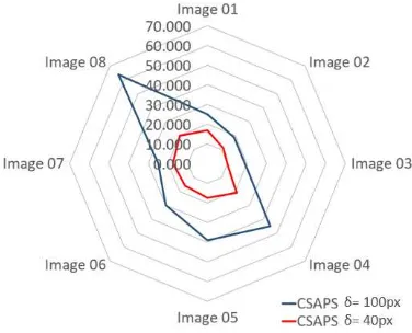
rately the system localizes center is made by calculating the root mean square of the deviations of true detections from object cen-ters as discussed in Section 2.5.3. The localization error of CAPS in case ofδ=40px is less than 20px and 70px for allowedδ = 100px. The maximum localization error occurs for Image 08, for which accuracy of detection is also worst. Except image 08 forδ=100px, all other images have localization accuracy below 50px, which is half of the allowed error. Furthermore, during the feature map derivation, the shift along rows and columns are carried out in an interval of 5 pixels, which also contribute signifi-cantly to the degradation of the locational accuracy of detections. The locational accuracy can be increased by decreasing this shift-ing step, but it will also make the process inefficient.
Figure 15: RMS localization error [pixels]
6. CONCLUSION
The algorithm performed well with comparable accuracy with the results from different authors, given that the test sites were chosen focusing on different challenges. Overall accuracy of the method for all test images is 84% forδ = 100pxand 76.1% forδ = 40px. Although, the performance of the algorithm was poor for few images, in most of the cases it produced results with high accuracies, despite the fact that training samples for algorithm were chosen only from the first scene.
CAPS as the feature was able to distinguish between palm trees and non-palm objects. But yet, few interesting false objects were detected, which had high CAPS values. It signifies that CAPS can also be used for recognition of different shapes, especially regular shapes, which also have high values of CAPS.
One drawback of CAPS is that its extraction is a non-linear pro-cess, and hence, the efficiency of feature extraction is low. Fur-ther study on increasing the efficiency would strengthen the fea-ture. Finally, CAPS proved to be a shape feature that distin-guishes palm trees that can be used singularly in object detection.
However, for increased accuracy, it also can be used in combina-tion with other features.
7. ACKNOWLEDGEMENTS
We would like to acknowledge Trimble Navigation Ltd. for the generous help in the study. The organization supported the project by contributing the UAV images and technical resources for the experiment. We would like to especially thank Mr. Roland Win-kler and Dr. Barbara Zenger-Landolt for advising, supporting and giving feedbacks throughout the study.
REFERENCES
Ben-Hur, A. and Weston, J., 2010. A user’s guide to support vector machines. In: Data mining techniques for the life sciences, Springer, pp. 223–239.
Bishop, C. M., 2006. Pattern Recognition and Machine Learning (Information Science and Statistics). Springer-Verlag New York, Inc., Secaucus, NJ, USA.
Chang, C.-C. and Lin, C.-J., 2011. Libsvm: A library for support vector machines. ACM Transactions on Intelligent Systems and Technology (TIST) 2(3), pp. 27.
Colchester, M., 2011. Oil palm expansion in South East Asia: trends and implications for local communities and indigenous peoples. Forest Peoples Programme.
Cortes, C. and Vapnik, V., 1995. Support-vector networks. Ma-chine learning 20(3), pp. 273–297.
Economy, G., Potts, J., Lynch, M., Wilkings, A., Hupp´e, G., Cun-ningham, M. and Voora, V., 2014. The state of sustainability ini-tiatives review.
Food & Agriculture Organization of United Nation, 1977. The oil palm. FAO Economic and Social Development Series.
Jusoff, K. and Pathan, M., 2009. Mapping of individual oil palm trees using airborne hyperspectral sensing: an overview. Applied Physics Research 1(1), pp. 15–30.
Liu, X., Gao, C. and Li, P., 2012. A comparative analysis of support vector machines and extreme learning machines. Neural Networks 33, pp. 58–66.
Malek, S., Bazi, Y., Alajlan, N., AlHichri, H. and Melgani, F., 2014. Efficient framework for palm tree detection in uav images. IEEE Journal of Selected Topics in Applied Earth Observations and Remote Sensing 7(12), pp. 4692–4703.
Powers, D. M., 2011. Evaluation: from precision, recall and f-measure to roc, informedness, markedness and correlation. Jour-nal of Machine Learning Technologies 2(1), pp. 37–63.
Srestasathiern, P. and Rakwatin, P., 2014. Oil palm tree detec-tion with high resoludetec-tion multi-spectral satellite imagery. Remote Sensing 6(10), pp. 9749–9774.
Suykens, J. A. and Vandewalle, J., 1999. Least squares sup-port vector machine classifiers. Neural processing letters 9(3), pp. 293–300.
Taza, A. and Suen, C. Y., 1989. Discrimination of planar shapes using shape matrices. IEEE Transactions on Systems, Man and Cybernetics 19(5), pp. 1281–1289.