APPLICATION OF LIDAR-DERIVED DEM FOR DETECTION
OF MASS MOVEMENTS ON A LANDSLIDE
M. Barbarella a, M. Fiani b, A. Lugli a
a
DICAM, Università di Bologna, Viale Risorgimento 2, 40136 Bologna, Italy – (andrea.lugli8, maurizio.barbarella)@unibo.it
b
DICIV, Università di Salerno, Via Ponte Don Melillo 1, 84084 Fisciano (SA), Italy - [email protected]
KEY WORDS:TLS, Landslides, Hazard, Monitoring, DEM/DTM, Georeferencing, Segmentation, Point Cloud
ABSTRACT:
In order to reliably detect changes in the surficial morphology of a landslide, measurements performed at the different epochs being compared have to comply with certain characteristics such as allowing the reconstruction of the surface from acquired points and a resolution sufficiently high to provide a proper description of details. Terrestrial Laser Scanning survey enables to acquire large amounts of data and therefore potentially allows knowing even small details of a landslide. By appropriate additional field measurements, point clouds can be referenced to a common reference systemwith high accuracy,so thatscans effectively share the samesystem.In this note we present the monitoring of a large landslide by two surveys carried out two years apart from each other.The adopted reference frame consists of a network of GNSS (Global Navigation Satellite Systems) permanent stations that constitutes a system of controlled stability over time.Knowledge of the shape of the surface comes from the generation of a DEM (Digital Elevation Model).Some algorithms are compared and the analysis is performed by means of the evaluation of some statistical parameters using cross-validation.In general, evaluation of mass displacements occurred between two surveys is possible differencing the corresponding DEMs, but then arises the need to distinguish the different behaviors of the various landslide bodies that could be present among the slope.Here landslide bodies‟ identification has been carried out considering geomorphological criteria, making also use of DEM derived products, such as contour maps, slope and aspect maps.
1. INTRODUCTION
Many geomatic techniques offer the possibility of acquiring 3D information of the terrain with high accuracy and high spatial resolution.Geomatic techniques give a great contribution to the knowledge of both the surface shape and the kinematics of landslides providing data which can be used by geologists, geomorphologists and geotechnics for interpreting the phenomenon.
In particular LiDAR technique is very interesting for its applications in landslide hazard analysis thanks to its ability to produce accurate and precise digital elevation models (DEM) of land surface. Especially the terrestrial laser scanners have the advantage to provide huge amounts of data at high resolution in a very short time and then they allow a precise and detailed description of the scanned area (Slob and Hack, 2004; Pirotti et al. 2013a).A detailed overview of LiDAR techniques applied to landslides is contained in Jaboyedoff et al. (2012).
Main applications to the landslides range from mapping and characterization (Guzzetti et al., 2012; Derron M.H. and Jaboyedoff M., 2010) to monitoring (Abellan et al., 2009; 2010; Barbarella and Fiani, 2012; 2013a,b; Prokop et Panholzer, 2009; Teza et al., 2007).
To obtain a digital terrain model (DTM) it is essential to extract the bare soil data from the whole dataset.The editing of the data requires a large amount of work; without this however it is not possible to use the data for a quantitative precise analysis of the movements of the soil.This task consists of a classification of the data coming from laser scanners into terrain and off-terrain ones. Due to the huge amount of data that is generated by the laser scanning technique, there is a need to automate the process. A detailed overview of both several filter algorithms which have been developed for this task and a representative selection of some methods is contained in Briese (2010). The TLSs belonging to the last generation of instruments allow
acquiring more echoes; for example Riegl VZ series instruments are full waveform systems. They can provide, if properly equipped with software tools, a full waveform analysis very effective for the filtering of the vegetation (Elseberg et al, 2011; Guarnieri et al, 2012; Mallet and Bretar, 2009; Pirotti et al., 2013b; Pirotti et al., 2013c).
Subsequently, it is necessary to convert the irregularly spaced point data into a DEM which can be generated by appropriate interpolation methods (Kraus and Pfeifer, 2001; Vosselman and Sithole, 2004; Pfeifer and Mandlburger, 2009). The accuracy of a DEM and its ability to faithfully represent the surface depends indeed on both the terrain morphology and the sampling density but also on the interpolation algorithm (Aguilar et al., 2005, Barbarella et al., 2013b).
If the goal of survey is monitoring the ground deformation over time two or more DEMs have to be compared in order to monitor the displacements of a number of points of the terrain (Fiani and Siani, 2005, Abellan et al., 2009). Here a number of different approaches can be used. For examples one can directly compare the DEMs obtained over time by simply fixing a number of points belonging to particular objects visible in the two different point clouds (Ujike and Takagi, 2004); the estimated transform parameters can then be used in order to transform all the points of a cloud in the reference system of the other one, making possible a comparison between them (Hesse and Stramm, 2004).
A more general approach allowing a full three-dimensional analysis useful for point clouds comparison is based on the algorithm called LS3D, proposed by Gruen and Akca (2005). In this paper we describe the approach we used for TLS surveying and data processing in a “real world” study case, i.e. a large landslide that presents many criticalities in the monitoring over time.
belonging to the network established for real time surveyNRTK. These stations are monitored in continuous and are now widely used in many countries. A GNSS survey now is easy to do and it is not expensive. Since the permanent stations are far away from the landslide area, the baseline error is not so small; nevertheless, it is doubtlessly acceptable if you thinkthe increaseofaccuracy dueto the stabilityof areference system which is monitoredover timeon wideareas.
With regard to the reconstruction of a grid starting from the point clouds, given the importance to identify the best algorithm, we made a number of tests on a check sample extracted from the whole point clouds. We present the result of the comparison of various surface fitting algorithms in order to evaluate the quality of the interpolation in our operational context (taking into account both the terrain morphology and the huge density of points).
Finally, for the comparison between the surfaces of the terrain in two different epochs, to obtain the volume of the soil mass moved, we underline the need to segment the surface in a number of homogeneous areas to enable a quantitative analysis of the movements occurred over time.
At this stage, it is necessary to conduct a geomorphological study to better interpret the phenomenon in progress; geomorphologists may be assisted by products derived from the DTM, such as both contour maps and maps of slope and aspect. The evaluation of the soil volume moved over time is more accurate if the ground surface has been previously segmented.
2. METHOD AND MATERIALS
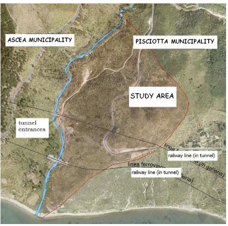
The phenomenon we are considering is taking place in Pisciotta municipality (Campania Region, Italy), on the left side of the final portion of the Fiumicello stream (figure 1).
Figure 1.Geographic location of landslide
The landslide causes extensive damage to both an important state road and to two sections of the railway line connecting North and South Italy (close to its East coast).
According to the widely accepted and used definition for landslide as „„the movement of a mass of rock, debris or earth down a slope‟‟ established by Cruden (1991) and Cruden and Varnes (1996), the active Pisciotta landslide is defined of “type
slow” and the movement of the soil is of the sliding rotational type, with the typical slipping that occurs along deep surfaces (Coico et Al., 2011).
In figure 2 we show an excerpt from the geological map; the rocks are a mix of “marnoso-arenacee”, calcareous and clayey of the Cilento flysch.
Figure 2. Excerpt from the geological map of Campania region(http://webgis.difesa.suolo.regione.campania.it/website/D
S2/viewer.htm?dservice=geoapat)
In the period 2005-2009 two traditional topographical surveys per month were performed by materializing a set of vertexes on the landslide body and controlling its position.
These operations, carried out by Iside Srl group on behalf of “Provincia di Salerno”, allowed a first estimate of the magnitude of the ground movement, but such a control network is not sufficient to describe mass movements and changes in the shape of the slope.
In order to obtain a 3D numerical model of the landslide slope and its variation over time we run a number of surveying campaigns using Terrestrial Laser Scanning surveying methodology (Barbarella and Fiani, 2012, 2013a,b).
We carried out a TLS “zero” survey and about four months later a repetition measurement using a long-range instrument, Optech Ilris 36D; a further surveying campaign was carried out one year later by using two different instruments, a long range (Riegl VZ400) and a medium range one (Leica Scanstation C10). The last campaign dates back to June 2012. Here we used both Optech and Leica instruments.
Inall our survey campaigns we have recorded laser scan measurements coming from a number of TLS stations, located on the stable slope at different altitudes, so to measure boththeupper and thelower partof thelandslide, down to the stream; here the distance are smaller and short range instruments can be used, obtaining a larger density of points. In the lower part of the ridge there is a railway bridge and the terrain above the entrance of the tunnel can be measured with high accuracy; not far fromthis, towards the valley,there is alonger bridgeand a tunnel.
in the neighborhood or inside the surveyed area, they can be used for georeferencing all the scans and thus make the surveys comparable. If no detail within the point cloud may be considered undoubtedly stable, the need to refer the surveys to stable areas arises.
Once all the point clouds are framed in a common reference system, we can compare them over time. To do this we need a digital elevation model that represents the earth‟s surface. The DEMs can be in the form of Triangulated Irregular Network (TIN) or grid. While TINs are generally built applying the Delaunay criterion, in order to create a grid we have to choose an interpolation algorithm to calculate the grid node values starting from the sparse point clouds. The accuracy of a DEM and its ability to faithfully represent the surface depends on both the terrain morphology and the sampling density but also on the interpolation algorithm (Aguilar et al., 2005; Fiani and Troisi, 1999; Kraus et al., 2006; Pfeifer and Mandlburger, 2009). We performed a number of tests to compare the surfaces built using several DEM interpolation methods on the same sampleofdata.
2.1 Georeferencing by means of GNSS permanent network In our case study the only detail in the whole scene which can give us some assurance of stability over time is the entrance of the tunnel on the lower part of the landslide. It is nevertheless not large enough and it is too peripheral in the scan to guarantee a correct georeferencing of the whole area.
Therefore, it is necessary to adopt a reference frame locatedin a stable area and close enough to simplify the survey. For this purpose, wehave considered two pillars materialized in front of the landslide, from which we have measured the position of the targets necessaryforgeoreferencing the scans, using GPS receivers.Since the whole area surrounding the landslide does not give full guarantee of stability, these two pillars have been connected to two vertices belonging to the network of GNSS permanent stations for NRTK survey, that are continuously monitored in the ITRS system. The permanent stations are about 30-40 km far away, but the increase in error due to the greater distance in the frame is largely offset by the guarantee of stability over time.
Both the bridge and the mouth of the tunnel do not show any evidence of deformation occurred. So they can be used as stable details to check on them the absolute georeferencing of the data coming from the two periods, allowing us to estimate the local shift. This is probably due to the error in the estimation of the baselines between the pillars and the fixed points that are far away. We have been able to evaluate the amount of the difference of the position of the samedetail by comparing the coordinates of a number of “homologous” pointsidentifiedon theartifact. The coordinate differences between the very fewpoints really “homologues” belonging to the twoscans (2012 and 2010) reached 6, 4, 4 cm average respectively in the North, East and height components, with standard deviations of the means of 2 cm on average for all the three coordinates. The comparisonbetween the heights of the points located on the top of the tunnelconfirmed the magnitude of the coordinate differences.We therefore could evaluate the overall georeferencing error (locally) well within 10 cm. It is not possible to cancel this error but we can reduce its effect performing a rigid body transformation, i.e. a translation of the amount previously found. We made this before the comparison between scans. Then we made the comparison in order to obtain the differences over time between both surfaces and volumes or the profiles, we should therefore take in account an uncertainty in the coordinates of the order of nearly 5 cm, due to thegeo-referencing step.
2.2 Choice of surface interpolation algorithm
There are many interpolation algorithms for generating surface grid based DEM. In landslide analysis the choice of the algorithm is not obvious, depending on various factors such as terrain morphology and presence of discontinuities. The assessment of the surface deformation occurred over time is strongly influenced by the DEM construction mode.
Frequently used algorithms implemented in most widespread software are: Inverse distance to a power, Kriging, Natural Neighbor, Nearest Neighbor, Local Polynomial, Radial Basis Function. We chose some of these interpolators to perform a test on the lower part of the landslide, which is characterized by the presence of discontinuities, of an artifact (the mouth of a tunnel) and is practically deprived of vegetation. (figure 10) For the choice of the interpolator we used a very simple criterion, i.e. the degree of adherence of the interpolated surface to the original data used to generate the surface. For this we calculated the deviation of the laser points from the interpolated surface. The difference between the height zk of the point and the interpolated height zint(xk,yk) is here called residual. We used a method of cross-validation, extracting from the sample of 4 million points a sub-sample of 1% of points (N=40,000) extracted by decimation.
We then calculated the height differences between the N points belonging to this check sample and the interpolated surface generated considering the remaining 99 percent of the data. For the modeling of the surface, in particular, we used the algorithms and associated parameters reported in table 3.
ALGORITHM PARAMETER ACRONYM
Inverse distance to a power 2nd degree Idw2
Kriging linear variogram Kri
Natural Neighbor NatNe
Table 3. Algorithms tested in an area with artifacts, terrain discontinuities but practically deprived of vegetation
If we consider the standardized residuals u, i.e.: ( x
) /
xu
x m
s
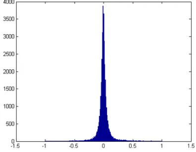
The corresponding histogram is shown in figure 5superimposed with the probability density function of a standardized normal distribution N(0,1).
Figure 4. Histogram of the sample of the residuals obtained by cross-validation using the IDW2 algorithm
Figure 5. Histogram of the relative frequency of the standardized residuals using the Idw2 algorithm and of the standardized normal distribution. The departure from the normal
distribution is quite evident
It is very hard to consider the residuals of the interpolations to be normally distributed, regardless the algorithm tested. To evaluate and parameterize differences among the algorithms we calculated some statistical parameters, the most traditional (mean m, root mean square error), but also third and fourth standardized moments (skewness g1 and kurtosis g2), and robust parameters of centrality and dispersion (median, median absolute deviation ). As is well known, the median can be computed as the central value in the ascending ordered sample (or the average of the two central values, if the number N is even).
The analytical expressions of the aforementioned statistics are:
2 obtained for these parameters are shown in table 6.
ALGORITHM MEAN
Table 6. Some statistical parameters for the tested interpolation algorithms (rmse: root mean square error; mad: median absolute
deviation)
The statistical parameters are not very different among the algorithms.rmse ranging from13 to 15 cm and the mad from 2.9 to 3.7 cm, the means from 0.3 to 0.5 cm.
If we compare the algorithms in terms of capacity to describe the terrain, the best results are given by Idw2, Local Polynomial and Radial Basis Function (with smoothing factor c2=0), even if the differences between them are substantially quite small. However, the best overall performance is provided by Idw2 which has been chosen for subsequent elaborations. This method also allows introducing breaklines to better characterize the trend of the ground (Lichtenstein and Doytsher, 2004) especially in the vicinity of the artefacts. For these reasons we chose the algorithm Inverse distance to a power in order to get the interpolated surface of the landslide.
With regard to the Radial Basis Function, must be studied in more detail the influence of the value adopted for the smoothing factor, as the first results were conflicting.
A few remarks about the statistical characteristics of the samples of residuals, valid for all interpolators; the distributions:
- are almost symmetrical, in general algorithms present a slight longer tail to the right (are skewed right) more or less pronounced;
- are strongly leptokurtic: have values of excess kurtosis very high;
- have a ratio rmse / mad very high, compared to what would compete to a normal distribution (about 1.5).
To conclude, the following analysis is referred to a grid DEM built by means of Idw2 algorithm; we designed the breaklines only in correspondence of the mouth of the tunnel, which is the sole artefact present in the scans.
3. RESULTS
pillars (Iside100 and Iside200), of the TLS station points (LS1 and LS2) and of the targets (T1÷T11) for the 2010 survey.
Figure 7. 2010 survey. We show the location of “near reference” pillars (in red), laser scanner stations (in orange) and
targets (in green)
In each scan we use a number of targets in order to frame the whole survey in a unique reference system. Both the target and the TLS station coordinates were measured by GNSS instruments in static mode keeping fixed the coordinates of two pillars placed on the opposite side of the valley. The scheme of GNSS survey is shown in figure 8.
Figure 8. Scheme of the survey of the target from the two pillars by GNSS bases (date of the survey:02/25/2010)
The result of the GPS baselines adjustment has provided values for the target coordinatesin 2010: the rmse was on average less than 1 cm both in planimetry and in altimetry, but was higher in height, about 4 cm.
For the data coming from TLS we performed all the processing steps, namely scans alignment, editing and georeferencing using Polyworks software package.We made a 6 parameter transformation in order to georeferencing all the scans; a 7 parameters transformation (conformal transformation) gives almost the same results. We note that usually the laser data processing software packages do not provide a rigorous analysis of the quality of the standardized residuals of the transformation. The process of georeferencing has led to values of 3D residuals ranging from 5 to 6 cm.
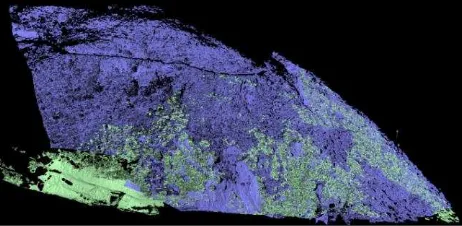
In figure 9 we show the aligned and georeferencing points cloud obtained in 2012 surveying campaign.
Once these steps have been done two point clouds which describe the landslide surface in two different epochs are available. Since all the surveys have been framed in the same reference system, it will be possible to compare the DTMs elaborated starting from the point clouds obtained at different times.results.
Figure 9. Whole points cloud obtained in 2012
A first comparison between the two point clouds could be performed considering as a reference surface the interpolated mesh of one of the two clouds. In order to follow the evolution of the landslide morphology here it has been chosen to consider the 2010 surface as the reference one. The “Compare” procedure implemented in PolyWorks consists in measuring the distance of each point of a cloud with respect to a reference surface.
Here it has been chosen to measure distances along the shortest path from the point to the surface. The sign of the distance depends on the relative position of cloud and mesh: if a point is above the mesh the distance is positive (in this case it corresponds to accumulation of debris, represented from yellow to brown in figure 10), otherwise, if it is below the mesh, the sign is negative (“erosion”, from light to dark green, the meaning of the term “erosion” will be better explained in the following).
At the end of process, input data points are represented in a chromatic scale whose entities correspond to the distance values.
Figure 10. Comparison of 2012 points cloud with respect to the 2010 reference mesh in a sample area located in the nearby of the railway tunnel. Palette: points with colorsfrom dark to light
green correspond to “erosion” areas, points from yellow to brown to accumulation ones
3.1 Classification
The results of a comparison procedure like this are suitable for a quick identification of stable/unstable areas but do not allow performing metric estimates of mobilized volumes.
In the study of a landslide, an important information refers to the amount of debris mobilized in a certain period. In commercial software packages oriented to TLS data processing this result is often achieved differencing the volumes comprised between the interpolated surfaces and a horizontal reference plane.
In order to get a quantitative estimation of mobilized volumes in terms of loss and gain here it has been chosen to perform
Iside200 Iside100
Ls1
T7
T9
T10
T11 T4
T5
T6
T6bis T2
T3
T8
T1
Ls2
-calculations differencing in a GIS environment the DTM grids derived from both the two scans.
The two point clouds have been first interpolated with Idw2, and 50 cm cell width. The cell width has been chosen accordingly to the mean span of the points in both the surveys. The grids corresponding to interpolated surfaces have then been differenced, subtracting the 2010 one to the 2012 one
This elaboration has been performed in a GIS environment using a raster calculator (analogous results have been obtained in ArcGIS considering TINs, using a surface difference tool). To distinguish areas in erosion from those of accumulation, the resulting grid has been classified into three classes (figure 11): -from -0.1 m to 0.1 m, representing areas which could be
considered as characterized by the balance of loss and gain (for sake of simplicity in the following these points will be defined just as “stable”)
-equal or greater than 0.1 m, areas in accumulation from 2010 to 2012 (e.g. 2012 surface is above the 2010 one);
-equal or lower than -0.1 m, areas in “erosion” (e.g. 2012 surface is below the 2010 one).
Figure 11. Automatic segmentation into three classes of the grid obtained subtracting the 2010 DTM to the 2012 one. In green
are represented cells corresponding to accumulation, in red those corresponding to “erosion” and in yellow those that could
be considered as “stable”
The threshold of 10 cm for stable/unstable points corresponds to a rough estimate of the overall precision of the method (deriving from alignment, georeferencing, interpolation and comparison accuracy).
It has to be noted that the difference values in points corresponding to railway tracks are around zero: given the
intrinsic stability of the tracks this fact could be considered as an evidence of georeferencing quality and correction shift appropriateness.
The term “erosion” here should not been interpreted only as landslide displacement or as weathering, but also as an effect of removal of landslide debris which could dam the Fiumicello stream and the nearby gravel road.
The area around the tunnel has not been considered in calculations, in order not to affect the results with spurious differences deriving from the different acquisition geometries of the two scans. As previously mentioned, railway tunnel and tracks could be considered the only stable part of all the scenery. As expected, “stable” points are located near the railway tunnel and between accumulation and erosion areas. These results are in agreement with the comparison performed in PolyWorks, taking into account the different directions considered in calculations (along the vertical in DTM comparison, along the shortest path from the point to the reference mesh in PolyWorks).
This classification into only three classes represents a sort of rough segmentation, which would had been the proper way to study the landslide in all its aspects but it would have required specific algorithms.
Anyway information related to the global volume could be not representative of relative displacements between portions of the landslide.
For this reason it is advisable to perform volume calculations considering homogenous areas with respect to the relative position (below/above) of the two surfaces.
3.2 Landslide’s bodies identification
Volumes mobilized over the two years have first been calculated on the entire part of the landslide common to the two surveys, resulting in 58820 m3
of total accumulation and 48851
m3 of total “erosion”, mainly due to excavation. The total
volume corresponding to points considered as stable (from -0.1 m to 0.1 m of difference) is about 235 m3.
This approach is obviously not exhaustive because consider the landslide as a whole body does not allow an analysis of the evolution in time of its shape. For this reason it is important to segment the landslide in its different bodies, so as to able to perform a more articulated volumes calculation, definitely more significant.
To make a classification that allows these analyses it has been necessary to recourse to a geomorphologists expert in Pisciotta landslide area, who has been able to draw the different polygons to be analyzed on the basis of DEM derived products supplied by us (Guida D,. 2013, personal communication).
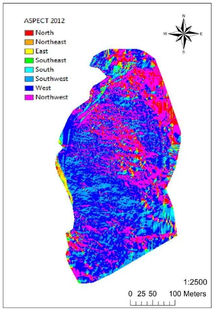
More in detail, for both the epochs we have provided the consulted geomorphologist with contour maps with small intervals (up to 0.25 m), slope maps and aspect maps.
All these products have been derived from DEMs interpolated with a spacing of 0.50 m.
Slope and aspect maps are shown in figures 12-15. Contour map derived from the TLS survey performed in 2010 with the various landslide bodies in overlap is shown in figure 16. The morphological analysis showed that the slope under study (orographic left bank) is affected by landslides that differ by type, age and stage of activity. On the main body of the landslide in fact it is possible to recognize landslides of second and third generation. The phenomenon is characterized by a slow roto-translational behavior in the upper part, evolving downward in slides and clay flows.
Figure 12. Slope map derived from 2010 TLS survey. Slopes have been classified into 6 classes from 0° to 65°; upper
slopes are merged into a single class
Figure 13. Aspect map derived from the 2010 survey, classified into 8 classes corresponding to cardinal direction
Figure 14. Slope map derived from 2012 TLS survey. Slopes have been classified into 6 classes from 0° to 65°; upper
slopes are merged into a single class
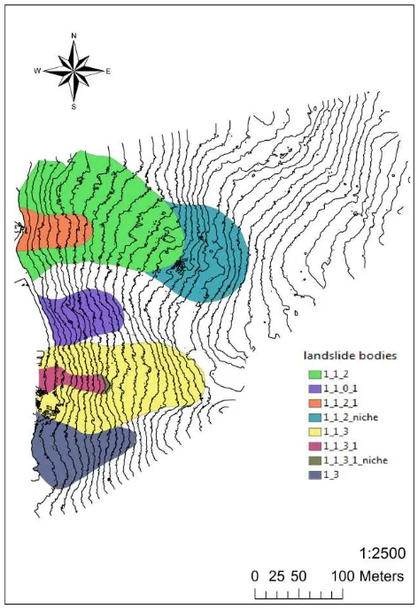
Figure 16. Contour map derived from the TLS survey performed in 2010 (which has been assumed as the reference one) with the various landslide bodies in overlap; for sake of
clarity here lines are represented with an interval of 5m
On the whole, it is possible to identify six polygons that represent:
- a landslide of second generation indicated by the abbreviation "1_3"
- two landslides of third generation indicated by the abbreviations"1_1_2" and "1_1_3"
- three landslides of fourth generation classified as "1_1_0_1", "1_1_2_1", "1_1_3_1" in analogy with the previous ones The main body of the landslide, which would have been indicated by the abbreviation "1", is not visible in figure 16, as well as the third generation landslide body classified as "1_1_0", because their extension exceeds the area detected by the TLS survey in 2010.
With regard to these different landslide bodies identified throughout the landslide, volume calculations have been performed considering only two classes, erosion and accumulation.
More in detail, for each landslide body have been calculated both its aggregated volume and both volumes corresponding to erosion and accumulation zones, reported in table 17.
Table 17.Volumes mobilized from 2010 to 2012 in identified landslide bodies
3.3 Variations over time of landslide bodies’ shape
In general, there is a good correspondence between volume losses and gains between the several landslide bodies.
For instance, crown 1_1_2 shows a volume loss/gain balance which could be related to the volume gained by below areas. It is important to point out that the shapes of landslide bodies have been detected considering the 2010 contour map: in 2012 these features were probably different and so volume calculation estimates should be considered as affected by a certain level of uncertainty.
Moreover, human interventions that took place in 2011 in order to stabilize the toe of the landslide do not allow a clear interpretation of its behavior: 1_1_2_1 area shows a total loss of about four hundreds of cubic meters in spite of a noticeable loss of the above landslide bodies.
In 2011, the blocks of the retaining wall on the right of the tunnel were removed and repositioned, passing from three to five rows. This change is not clearly noticeable in the comparison results, probably because the surface of the reference mesh is continuous and more or less the blocks are positioned along the steepness of the slope.
Only a few anomalies are pointed out by some patches clearly different from the surrounding areas, with irregular shapes not corresponding with the geometry of an ashlar (figure 18).
Figure 18. Comparison results over the ashlars nearby the railway tunnel
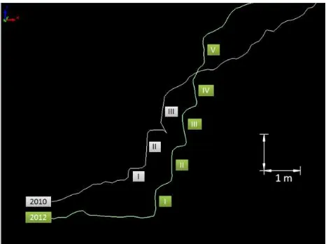
A clear evidence of this intervention in 1_1_2_1 area can be found also comparing profiles taken over the two scans, for instance blocks of the retaining wall on the right of the railway tunnel were removed and repositioned, passing from three to five rows. In figure 19 is shown a cross-section taken along the blocks of the retaining wall close to the railway tunnel.
NAME Area
(m2)
Vol ume (m3)
Area (m2)
Vol ume (m3)
Area (m2)
Vol ume (m3)
1_1_0_1 3758 4767 615 -308 4373 4458
1_1_2 13275 12953 6040 -5243 19315 7711
1_1_2_ni che 3982 5404 3844 -6659 7826 -1255
1_1_3 7908 7587 7230 -6675 15138 912
1_3 3990 7703 1770 -1248 5760 6455
1_1_2_1 1564 1290 1511 -1688 3075 -398
1_1_3_1 1024 765 375 -168 1400 597
1_1_3_1_ni che 103 121 27 -25 130 96
Figure 19. Cross-section taken along the blocks of the retaining wall close to the railway tunnel
4. CONCLUSIONS
TLS monitoring of a landslide is affected by some critical issues, the first of which is georeferencing.
As a matter of fact, there is the need to refer all the surveys acquired at different epochs to a unique reference system stable in time: if there is no stable detail inside the cloud with these characteristics, it could be more convenient to assume points located outside of the cloud, also quite far but really stable. Given the lack of stable reference benchmarks nearby the landslide, georeferencing could be made with respect to Continuously Operating Reference Stations, today presents in many countries, which are continuously monitored over wide areas for their intrinsic consistency.
Connection to targets by GNSS receivers implies some uncertainness in the determination of point positions, in this case about 5 cm in each coordinate; this estimate has been assessed considering the difference in positions of homologous points in the two surveys identified in the only stable object present in the scenery, the railway tunnel.
Another critical step is represented by the processing of the acquired clouds, that is undoubtedly the most time consuming task of the entire work, not only for the coregistration of the several scans constituting each single cloud, but also for surface reconstruction from clouds.
In case of DEM production over a grid, it is worthwhile an evaluation of which algorithm allows the better interpolation of the scanned surface, depending on landslide morphology and on points density.
Several tests have been performed considering the altimetric residuals of a sub sample of points (1% of the total) with respect to the grid obtained by interpolation performed on the remaining 99% of sample points with the different algorithms. The distribution of the residuals, regardless to the algorithm used, is strongly leptokurtic, very different from the Normal one. To control the performance of the different algorithms tested, some sample statistics have been considered; we decided to use the Inverse Square Distance Weighted as the most suitable algorithm for the interpolation.
Displacements detection could be performed considering DEMs, both in TIN or in grid format: in order to obtain useful results for understanding the phenomenon.
For what concerns the displacements detection, to simply perform surface comparisons, it is possible the rendering a
cloud with a chromatic scale of point to mesh distances. A comparison procedure like this however does not always provide clearly interpretable results; for instance in our case the change in the shape of a wall formed by ashlars is not well noticeable, while the tracking of cross section allows a better interpretation of the occurred human intervention.
Once having differenced the two interpolated DEMs, to obtain a good reliability in the evaluation of the mass movements having occurred between the two surveys it is essential to segment the calculation according to the different characteristics presented by the various parts of the landslide.
The intervention of a geomorphologist expert in the area, supported by DEM derived products, such as contour maps, slope maps and aspect maps, has identified several landslide bodies and allowed the calculation of the volumes of moved materials for each of these bodies, for example between a niche and the landslide body below.
An attempt for an automation (even if only partial) in the segmentation of the difference grid still remains an open issue, mathematical calculations performed over DEMs could provide valuable information.
References
Abellan, A., Jaboyedoff, M., Oppikofer, T., Vilaplana, J. M., 2009. Detection of millimetric deformation using a terrestrial laser scanner: experiment and application to a rockfall event. Nat. Hazards Earth Syst. Sci., 9, 365–372, 2009.
Abellan, A., Vilaplana, J.M., Calvet, J., Blanchard, J., 2010. Detection and spatial prediction of rockfalls by means of terrestrial laser scanning modelling. Geomorphology, 119:162– 171.
Aguilar, F.J., Agüera, F., Aguilar, M.A., Carvaj, F., 2005. Effects of Terrain Morphology, Sampling Density, and Interpolation Methods on Grid DEM Accuracy. Photogrammetric Engineering & Remote Sensing, 71(7), pp. 805–816.
Barbarella, M., Fiani, M., 2012. Landslide monitoring using terrestrial laser scanner: georeferencing and canopy filtering issues in a case study. In: International Archives of the Photogrammetry, Remote Sensing and Spatial Information Sciences, ISPRS12(XXXIX-B5:157-162).
Barbarella, M., Fiani M., 2013a.Monitoring of large landslides by Terrestrial Laser Scanning techniques: field data collection and processing. European Journal of Remote Sensing, 46: 126-151. doi: http://dx.doi.org/10.5721/EuJRS20134608.
Barbarella, M., Fiani, M., Lugli, A. Landslide monitoring using multitemporal terrestrial laser scanning for ground displacement analysis. Geomatics, Natural Hazards and Risk, in press. Briese, C., 2010. Extraction of Digital Terrain Models. 2010. In: Airborne and Terrestrial Laser Scanning. Whittles Publishing, pp. 135 - 167.
Coico, P., Calcaterra, D., De Pippo, T., Di Martire, D., Guida, D., 2011. A preliminary perspective on landslide dams of Campania region, Italy. In: The Second World Landslide Forum Abstracts, WLF2 – 2011 – 0442.
Cruden, D.M, 1991. A very simple definition for a landslide. IAEG Bulletin, pp. 27–29.
processes. In: Landslides: investigation and mitigation (Special Report). National Research Council, Transportation and Research Board Special Report. Turner, A.K., Schuster, R.L. (eds), Washington, DC, USA, 247, pp. 36–75.
Derron, M.H., Jaboyedoff, M., 2010. Preface to the special issue. In: LIDAR and DEM techniques for landslides monitoring and characterization. Nat Hazards Earth SystSci, 10:1877– 1879.
Elseberg, J., Borrmann, D., Nuchter, A., 2011. Full Wave Analysis in 3D Laser Scans for Vegetation Detection in Urban Environments. In: Proceedings of the XXIII International Symposium on Information, Communication and Automation Technologies (ICAT).
Fiani, M., Troisi, S., 1999. DEM‟s comparison for the evaluation of landslide volume.In: Proceedings of ISPRS WG VI/3 International Cooperation and Technology Transfer, Parma, February 15 - 19, 1999, vol. XXXII, part 6/W7, pp. 236-243.
Fiani, M., Siani, N., 2005.Comparison of terrestrial laser scanners in production of DEMs for Cetara tower. In: The CIPA
International Archives for Documentation of Cultural Heritage,
Volume XX-2005, pp. 277-281.
Gruen, A., Akca, D., 2005. Least squares 3D surface and curve matching. ISPRS Journal of Photogrammetry and Remote Sensing, 59 (3), pp.151-174.
Guzzetti, F., Mondini, A.C., Cardinali, M., Fiorucci, F., Santangelo, M., Chang, K.T., 2012. Landslide inventory maps: New tools for an old problem. Earth-Science Reviews, 112 (2012), pp. 42–66.
Guarnieri, A., Pirotti, F., Vettore, A., 2012.Comparison of discrete return and waveform terrestrial laser scanning for dense vegetation filtering. In: International Archives of the Photogrammetry, Remote Sensing and Spatial Information Sciences, ISPRS12(XXXIX-B7:511-516).
Hesse, C., Stramm, H., 2004. Deformation measurements with laser scanners – possibilities and challenges. In:Proceedings of international symposium on modern technologies, education and professional practice in geodesy and related fields, Sofia, Bulgaria.
Jaboyedoff, M., Oppikofer, T., Abellan, A., Derron, M.H., Loye, A., Metzger, R., and Pedrazzini, A., 2012. Use of LIDAR in landslide investigations: a review (2012), Nat. Hazards, (2012) 61:5-28.
Kraus, K., Karel, W., Briese, C., Mandlburger, G., 2006. Local accuracy measures for Digital Terrain Models. The Photogrammetric Record, 21(116): 342–354.
Kraus, K., Pfeifer, N., 2001. Advanced DTM generation from LIDAR data.In: International Archives of the Photogrammetry, Remote Sensing and Spatial Information Sciences, XXXIV (Pt. 3/W4), pp. 23– 30.
Lichtenstein, A., Doytsher, Y., 2004. Geospatial Aspects of merging DTM with breaklines. In: Proceedings of FIG Working Week 2004, NSDI and Data Distribution, Athens, Greece, May 22-27, 2004.
Mallet, C., Bretar, F., 2009. Full-waveform topographic Lidar: State-of-the-art. ISPRS Journal of Photogrammetry and Remote
Sensing, Vol. 64, Issue 1, pp. 1-16.
Pfeifer, N., Mandlburger. G., 2009. LiDAR Data Filtering and DTM Generation. In: Topographic laser ranging and scanning. Principles and Processing.Ji Shan and Charles K. Toth (Eds.), Taylor and Francis.
Pirotti, F, Guarnieri, A, Vettore, A., 2013a. State of the art of ground and aerial laser scanning technologies for high-resolution topography of the earth surface. European Journal of Remote Sensing, 46:66-78. doi: 10.5721/EuJRS20134605.
Pirotti, F, Guarnieri, A., Vettore, A., 2013b. Ground filtering and vegetation mapping using multi-return terrestrial laser scanning. ISPRS Journal of Photogrammetry and Remote Sensing, 76:56-63. doi: 10.1016/j.isprsjprs.2012.08.003.
Pirotti, F., Guarnieri, A., Vettore, A., 2013c. Vegetation filtering of waveform terrestrial laser scanner data for DTM production. Applied Geomatics, 5:311-322. doi: 10.1007/s12518-013-0119-3.
Prokop, A., Panholzer, H., 2009. Assessing the capability of terrestrial laser scanning for monitoring slow moving landslides. Nat. Hazards Earth Syst. Sci., 9: 1921-1928. Slob., S, Hack, R., 2004. 3D terrestrial laser scanning as a new field measurement and monitoring technique. In: Engineering geology for infrastructure planning in Europe: a European perspective, Lectures Notes in Earth Sciences, Springer, Berlin/Heidelberg, 104:179–189.
Teza, G., Galgaro, A., Zaltron, N., Genevois, R., 2007. Terrestrial laser scanner to detect landslide displacement fields: a new approach. Int J Remote Sens, 28:3425–3446.
Ujike, K., Takagi, M., 2004. Measurement of landslide displacement by object extraction with ground based portable Lased Scanner. In: Proceedings of the 25th Asian Conference on Remote Sensing, 2004.
Vosselman, G., Sithole, G., 2004. Experimental comparison of filter algorithms for bare-Earth extraction from airborne laser scanning point clouds.ISPRS journal of photogrammetry and remote sensing, n. 1, 2004, pp. 85-101.