Hierarchical Regularization of Polygons for Photogrammetric Point Clouds of Oblique
Images
Linfu Xie a, c, d *, Han Hu b, d, Qing Zhu b, c, Bo Wu d, Yeting Zhang a
a State Key Laboratory of Information Engineering in Surveying Mapping and Remote Sensing, Wuhan University, P. O. Box C310,
129 Luoyu Road, Wuhan, Hubei, P. R. China - [email protected]
b Faculty of Geosciences and Environmental Engineering, Southwest Jiaotong University, Chengdu, Sichuan, PR China -
c Collaborative Innovation Center of Geospatial Technology, 129 Luoyu Road, Wuhan, Hubei, PR China -
d Department of Land Surveying & Geo-Informatics, The Hong Kong Polytechnic University, Hung Hom, Kowloon, Hong Kong -
KEY WORDS: 2D Polygon Regularization, Normal Reconstruction, Global Optimization
ABSTRACT:
Despite the success of multi-view stereo (MVS) reconstruction from massive oblique images in city scale, only point clouds and triangulated meshes are available from existing MVS pipelines, which are topologically defect laden, free of semantical information and hard to edit and manipulate interactively in further applications. On the other hand, 2D polygons and polygonal models are still the industrial standard. However, extraction of the 2D polygons from MVS point clouds is still a non-trivial task, given the fact that the boundaries of the detected planes are zigzagged and regularities, such as parallel and orthogonal, cannot preserve. Aiming to solve these issues, this paper proposes a hierarchical polygon regularization method for the photogrammetric point clouds from existing MVS pipelines, which comprises of local and global levels. After boundary points extraction, e.g. using alpha shapes, the local level is used to consolidate the original points, by refining the orientation and position of the points using linear priors. The points are then grouped into local segments by forward searching. In the global level, regularities are enforced through a labeling process, which encourage the segments share the same label and the same label represents segments are parallel or orthogonal. This is formulated as Markov Random Field and solved efficiently. Preliminary results are made with point clouds from aerial oblique images and compared with two classical regularization methods, which have revealed that the proposed method are more powerful in abstracting a single building and is promising for further 3D polygonal model reconstruction and GIS applications.
1. INTRODUCTION
Since the re-invention by Pictometry (Petrie, 2009), aerial oblique images have become a standard for various mapping applications (Rupnik et al., 2014). In photogrammetry and computer vision communities, the automatic orientation technology for aerial oblique images have been widely studied and developed, including feature points matching (Hu et al., 2015), bundle adjustment (Rupnik et al., 2015; Xie et al., 2016). In recent years, high density point cloud acquired by dense image matching (DIM) from oriented aerial oblique images have become a major data source for 3D mapping (Fritsch and Rothermel, 2013). The automatic classification and segmentation of point clouds have been explored extensively
(Rottensteiner et al., 2012), while plane detection algorithm from unorganized point clouds are rather effective (Schnabel et al., 2007; Poppinga et al., 2008), both of which lying a good fundament for automatic generation of high quality vector information for various GIS applications.
However, 2D polygons and polygonal models are still the industrial standard. The inherent deficiencies of DIM point clouds data put great challenges in generating polygons with high geometry accuracy (Ahmadabadian et al., 2013). As summarized by (Hu et al., 2016), the quality of photogrammetric point clouds is inferior to that of laser scanning in the level of noise and preservation of sharp features. The forward intersected point clouds suffer the problem of inaccuracy positioning at the edge of building planes due to
disparity discontinuities, sharp features may degenerate at edges. Extraction of the 2D polygons from MVS point clouds is still a non-trivial task, given the fact that the boundaries of the detected planes are zigzagged and regularities, such as parallel and orthogonal, cannot preserve (Arikan et al., 2013).
Yet, the geometry features along with the semantic information of manmade objects are promising to be utilized in polygon simplification and regularization. The integration of such common knowledge and information obtained from triangulated points may contribute to overcome the gap between data fidelity and model regularity (Jarząbek-Rychard and Borkowski, 2016).
Aiming at automatic producing high quality 2D polygons from noisy DIM point clouds of oriented aerial images, in this paper, we propose a hierarchical regularization method of 2D polygons for photogrammetric point clouds. We start from closed photogrammetric point sequence obtained by conducting alpha shapes algorithm in 2D space (Guo et al., 1997). Two stages of regularization are employed: the local stage and the global stage. In the local stage, we adopted the hypothesis that building outlines are piecewise smooth. The normal of initial boundaries points are first reconstructed and help to fit initial line segments. In the global stage, initial fitted line segments belong to same polygons are further regularized with each other through minimizing an energy function which measures both regularity and residuals from the grouped points. The virtue of the proposed method is producing highly regularized polygons considering both local smoothness and global uniformity,
making a good balance between data fidelity and model regularity.
2. METHOD 2.1 Overview
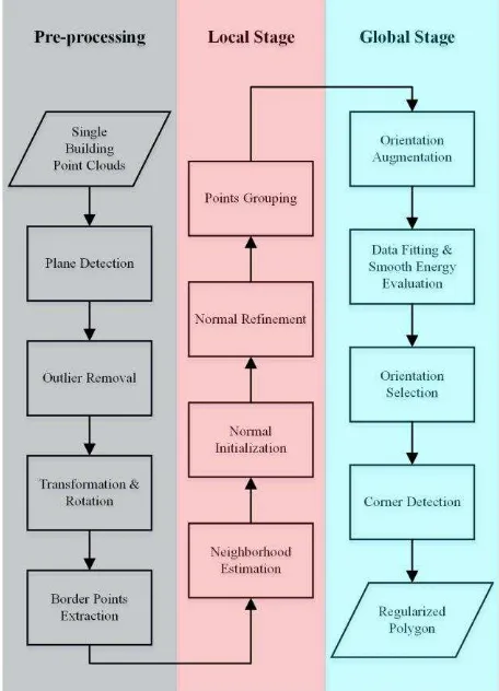
As shown in Figure 1, after pre-processing, the regularization are composed of two main stages: the local regularization stage and the global regularization stage. The objectives of the two stages are complementary. Closed point boundary are divided into piecewise smooth line segments in the local stage and global parallel and vertical relationship between line segments in overall area are discovered to further regularize edges and result in highly regularized polygons in the global stage.
Figure 1. Overview of the hierarchical regularization method
In the local stage, neighbouring relationship of consecutive building boundary points are build using a forward search strategy first, then the initial normal of each point are estimated by principal component analysis (PCA) with a fixed neighbour size. Based on the initial normal orientation and the neighbouring relationship, high quality 2D normal of each points are reconstructed by minimizing an least square function which decrease normal differences between neighbouring points while preserving final normal deviate too much from their initial value. The initial points are grouped according to the reconstructed normal and line segments with limited endpoints are fitted. These lines have finite extent that clipped to a bounding box based on the projection of points.
In the global stage, each line segment along with their mutable points are set as input to generate augmented line segments. The mutual parallel and vertical relation between each segments are used to form the augmentation. Then we construct an energy
function which consider both data fitting cost and overall smoothness using mutable points as observations. The energy function are minimized via graph-cut and result in highly regularized line segments in the global scene.
After two stage of refinement, the result polygons are generated through a simply corner detection method which merge line segments with the same orientation and intersect otherwise. In the following of this section, we describe the two stages in detail.
2.2 Local Stage
The goal of this stage is to robustly reconstruct for each boundary a piecewise smooth polygon that approximates the original outline. In order to achieve this goal, inspired by
(Avron et al., 2010), three steps which include neighbourhood estimation, normal refinement and points grouping are introduced, as illustrated in Figure 2.
Figure 2. Local stage regularization. (a) represent the alpha shapes boundary of plane; (b) represent the initial estimated 2D
normal of each point; (c) represent the refined 2D normal; (d) represent the reconstructed piecewise smooth polygon.
Neighbour relationship between points which belong to the same line are first estimated, then 2D normal are computed and refined based on the assumption that neighbour points are more likely to have uniform normal. After that, piecewise smooth polylines are grouped together in accordance with their 2D normal.
2.2.1 Neighbourhood Estimation: In this phase, the main purpose is to identify outlier-free collinear relationship between consecutive points. Hence a forward search based iterative method are used to estimate the neighbouring region. The neighbour region of a given points starts from one point (itself). In each iteration only one point (the next consecutive one) is added to this region if the residual of candidate point to the fitted least squares linear equation of the last iteration is below a given threshold. In order to strictly prevent outlier and preserve sharp features, a small threshold is preferred. The iteration stops when a candidate point is rejected, meanwhile, a new neighbour region detection starts. When all points have been allocated a neighbour region, normal refinement could be conducted.
2.2.2 Normal Refinement: Since 2D normal could be represent by rotation angles in 2D space, we transform the normal vector into angle space, which not only decrease the number of parameters but also promote the computational efficiency. In this phase, normal angle are initialized using existing method such as PCA analysis. Then a least squares cost function is formed based on the neighbouring relationship derived in the prior step. Two terms are incorporated as shown in Equation (1):
where N is the neighbour region; is the under refined normal angle and 0 is the initial value; is the scale factor. is the
weight between neighbouring points computed as followed:
where is pre-set parameter defining preferred angle difference which penalize big initial normal differences. The first term of Equation (1) minimizes the angle difference between neighbouring points while the second term restricts the normal angle deviate too much from their initial values. As depicted in Figure 2(c), after normal refinement normal angle differences at sharp features are enlarged while those in smooth region are reduced. The scale factor () is set to 0.1 and the preferred angle threshold () is set to 15 degree in our test datasets. As illustrated in Figure 2(b) and 2(c), point normal in smooth region become more identical with each other. In the meantime, abrupt normal changes occur around sharp features.
2.2.3 Points Grouping: Piecewise smooth polylines are constructed through grouping consecutive points which share similar normal angles since normal angle across sharp features are magnified in the previous step. In each grouped point set, a least squares line segment is generated and corners are detected by intersecting two consecutive line segments. As shown in Figure 3, the initial polygon boundary which consist of 416 points (black) is represented by a 17-edge polygon (red) that intersected from piecewise smooth point groups derived from our local regularization algorithm without losing primary sharp features.
Figure 3. Comparison between original points connected polygon and intersection polygon from grouped polylines.
2.3 Global Stage
Aiming at reconstruct regularized polygon with high fidelity, inter-polyline structure is explored since regulations are often enforced in manmade objects. In this stage, two principles are employed: (1) long line segments are better sample than short ones; (2) parallel and perpendicular relations should be discovered. Thus, this problem is generalized as an angle labelling problem, which could be formulated as Markov Random Field and solved via graph-cut algorithm efficiently
(Kolmogorov and Zabih, 2004).
For each line segments constructed in the local stage, the direction of its least squares line function has an orientation angle. Usually, this angle is almost orthometric with the average normal orientation of points that make up this line segment. In our hypothesis, line segments which constructed the same polygon may only have limited number of orientation angles, and these angles are always represented by larger segments. In other words, edges are encouraged to parallel or perpendicular with longer ones. Besides, the labelled angles should not deviate too much from its initial angles.
For these purposes, we first calculate all the orientation angles that appeared in the same polygon to form an angle set. Then each segment p is augmented by forming candidate line segments set (P) using the centre of the origin line and the orientation angles in Φ. After that an energy function considering both neighbour smoothness and data fitting degree is built to help segments to select proper orientation angles. Finally, line segments with same selected angles are merged and corners are detected. The energy function is shown in Equation (3). segments being labelled differently, N is the orientation neighbour region which includes pairs of line segments that have similar orientation angle; is the initial orientation angle of a given line segment; is the normalization angle value. Here, the initial orientation angle is augmented by simply including the perpendicular one.
In the second term, which measuring data fitting residuals, is the scale factor that balance the two term; D(p, θ) measures how well a line segment is fitting to the selected orientation angle, the computation is illustrated in Equation (4):
perpendicular distance from point i to candidate line segment p with orientation angle θ.
We implement the graph-cut algorithm (Boykov et al., 2001; Kolmogorov and Zabih, 2004) to minimize the energy function and convert the labelling result to the corresponding orientation angles. Successive segments with same orientations are merged to form a new one and corners are the intersection of two unparallel line segments. As depicted in Figure 4, after global stage regularization, the 17-edge piecewise smooth polygon are further merged and interested to form a 5-edge polygon
representing the main structure of the original point boundary while preserve the parallel and perpendicular relationship between main edges.
Figure 4. Comparison between original points connected polygon and final regularized polygon.
3. EXPERIMENTS 3.1 Test data description
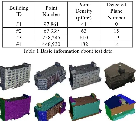
In order to test our algorithm, dense image matching point clouds of aerial oblique images are used. The datasets include urban areas in China and Zurich (Cavegn et al., 2014). For both datasets, image orientation and dense image matching are accomplished by existing solutions. After that, point clouds of some typical buildings are manually extracted by drawing a 2D bounding box, and planes are detected using a region growing based method (Adams and Bischof, 1994). For each single building, detected planes are first rotated and transformed into 2D space, then boarder points are extracted by applying the 2D alpha shapes algorithm.
Building ID
Point Number
Point Density
(pt/m2)
Detected Plane Number
#1 97,861 41 9
#2 67,939 63 15
#3 258,245 810 19
#4 448,930 182 14
Table 1.Basic information about test data
Figure 5. Point clouds and detected plans of test buildings. The building ID is corresponding to the column number, and he first
column shows the original point clouds while the second column illustrate detected planes by different colours.
We compared our algorithm with the traditional Douglas-Peuker algorithm and the polygon simplification algorithm implemented by CGAL (Dyken et al., 2009; Fabri and Pion, 2009). Both 2D and 3D comparison are presented and analysed.
The building under test are illustrated in Figure 5 and their base information are given in Table 1. In purpose of compare different polyline simplification algorithms objectively, we choose to compare the outcomes that representing a polygon by same number of vertexes.
3.2 Experimental Comparison
As shown in Figure 6-9, although all the three tested algorithm could simplify polygon outlines to certain degrees, the superiority of the proposed algorithm is obvious. For single polygon, sharp features are preserved, and the output of our method maintain the parallel and perpendicular relationship between edges. This virtual is magnify in building outline regularization because of the fact that horizontal and vertical structures are frequently appear in rooftops and facades. Compared with the other two simplification algorithms which may lose key points at sharp features, the proposed method represent these features concisely.
Figure 6. Regularization comparison on Building #1. The first, second, third row shows result from the proposed method, the Douglas-Peuker algorithm and Dyken’s method (Dyken et al., 2009)respectively. Results are compared in two complementary
views.
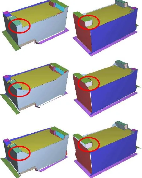
One the other hand, unlike main orientation based method, our method could handle polygons with different orientations correctly. Because in the global regularization stage, the orientation angle of an edge is not decided by either parallel or perpendicular to main edge, instead, it is selected in consideration of both data fitting residuals and inter-edge regularity. In Figure 7, it is clearly shown that the regularity of rectangles are concisely represented, meanwhile, data fidelity of other boundaries are reconstructed with high fidelity (e.g. the dark blue polygon).
Figure 7. Regularization comparison on Building #2. The figure arrangement are the same as Figure 6.
Although we have not yet consider regularity between different polygons with same building faces, the outcome of our algorithm achieve this virtue to some extent. As circled out in Figure 6-9, corners which shared by three different planes in object space could visually recognize in the final 3D polygon sets.
Figure 8. Regularization comparison on Building #3. The figure arrangement are the same as Figure 6.
This feature is potentially useful for topology reconstruction between polygons. Thus, subsequent automatic, or
semi-automatic, 3D model generation could benefit from this characteristic. In other words, the output polygons of the proposed method are more editable than polygons simplified by using traditional methods. Some polygons snapping algorithms could use the results of our algorithm as input (Arikan et al., 2013).
Figure 9. Regularization comparison on Building #4. The figure arrangement are the same as Figure 6.
4. CONCULTIONS AND FUTURE WORK In this paper, a hierarchical regularization of 2D polygons for photogrammetric point clouds of oblique images is presented. Two stages of regularization which reconstruct piecewise smooth line segments and global regularized polygons are incorporated. By comparing with existing polygon simplification algorithms the quality of the proposed method is verified, both fidelity and regularity are kept in our output polygons which lying a good foundation for subsequent 3D reconstruction.
In the future, two related problems should be solved. One is to robustly detect and consolidate planar robustly in noisy DIM point clouds, the other is to use the polygons obtained in this paper for polygonal mesh reconstruction through vertices snapping, such as OSnap (Arikan et. al., 2013) rather than the approach of volumetric segmentation or 3D plane arrangements, because in those approaches, vertex topologies will be lost.
ACKNOWLEDGEMENTS
This study was supported by the National Natural Science Foundation of China (Nos. 61602392, 41501421, 41631174 and 41571392). The authors would like to acknowledge the provision of the datasets by ISPRS and EuroSDR, released in conjunction with the ISPRS scientific initiative 2014 and 2015, lead by ISPRS ICWG I/Vb.
REFERENCES
Adams, R., Bischof, L., 1994. Seeded region growing. IEEE Transactions on Pattern Analysis and Machine Intelligence 16 (6), 641-647.
Ahmadabadian, A.H., Robson, S., Boehm, J., Shortis, M., Wenzel, K., Fritsch, D., 2013. A comparison of dense matching algorithms for scaled surface reconstruction using stereo camera rigs. ISPRS Journal of Photogrammetry and Remote Sensing 78, 157-167.
Arikan, M., Schwärzler, M., Flöry, S., Wimmer, M., Maierhofer, S., 2013. O-snap: Optimization-based snapping for modeling architecture. ACM Transactions on Graphics (TOG) 32 (1), 6.
Avron, H., Sharf, A., Greif, C., Cohen-Or, D., 2010. ℓ 1-Sparse reconstruction of sharp point set surfaces. ACM Transactions on Graphics (TOG) 29 (5), 135.
Boykov, Y., Veksler, O., Zabih, R., 2001. Fast approximate energy minimization via graph cuts. IEEE Transactions on Pattern Analysis and Machine Intelligence, 23 (11), 1222-1239.
Cavegn, S., Haala, N., Nebiker, S., Rothermel, M. & Tutzauer, P., 2014. Benchmarking High Density Image Matching for Oblique Airborne Imagery. In: Int. Arch. Photogramm. Remote Sens. Spatial Inf. Sci., Zurich, Switzerland, Vol. XL-3, pp. 45- 52.
Dyken, C., Dæhlen, M., Sevaldrud, T., 2009. Simultaneous curve simplification. Journal of Geographical Systems 11 (3), 273-289.
Fabri, A., Pion, S., 2009. CGAL: The computational geometry algorithms library. In: Proc. Proceedings of the 17th ACM SIGSPATIAL international conference on advances in geographic information systems, ACM, pp. 538-539.
Fritsch, D., Rothermel, M., 2013. Oblique image data processing - potential, experience and recommendation. In: Proc. Photogrammetric Week 2013, Stuttgart, Germany, 9-13 September, pp. 73-88.
Guo, B., Menon, J., Willette, B., 1997. Surface reconstruction using alpha shapes. In: Proc. Computer Graphics Forum, Wiley Online Library, pp. 177-190.
Hu, H., Chen, C., Wu, B., Yang, X., Zhu, Q., Ding, Y., 2016. TEXTURE-AWARE DENSE IMAGE MATCHING USING TERNARY CENSUS TRANSFORM. ISPRS Annals of Photogrammetry, Remote Sensing and Spatial Information Sciences, III-3, 59-66.
Hu, H., Zhu, Q., Du, Z., Zhang, Y., Ding, Y., 2015. Reliable spatial relationship constrained feature point matching of oblique aerial images. Photogrammetric Engineering and Remote Sensing, 81 (1), 49-58.
Jarząbek-Rychard, M., Borkowski, A., 2016. 3D building reconstruction from ALS data using unambiguous decomposition into elementary structures. ISPRS Journal of Photogrammetry and Remote Sensing, 118, 1-12.
Kolmogorov, V., Zabih, R., 2004. What Energy Functions Can Be Minimized via Graph Cuts? IEEE Transactions on Pattern Analysis & Machine Intelligence, 26 (2), 147-59.
Petrie, G., 2009. Systematic oblique aerial photography using multiple digital cameras. Photogrammetric Engineering and Remote Sensing, 75 (2), 102-107.
Poppinga, J., Vaskevicius, N., Birk, A., Pathak, K., 2008. Fast plane detection and polygonalization in noisy 3D range images. In: Proc. 2008 IEEE/RSJ International Conference on Intelligent Robots and Systems, IEEE, pp. 3378-3383.
Rottensteiner, F., Sohn, G., Jung, J., Gerke, M., Baillard, C., Benitez, S., Breitkopf, U., 2012. The ISPRS benchmark on urban object classification and 3D building reconstruction. ISPRS Ann. Photogramm. Remote Sens. Spat. Inf. Sci, 1, 3.
Rupnik, E., Nex, F., Remondino, F., 2014. Oblique multi-camera systems – orientation and dense matching issues. International Archives of the Photogrammetry, Remote Sensing and Spatial Information Sciences, 38 (W1), 107-114.
Rupnik, E., Nex, F., Toschi, I., Remondino, F., 2015. Aerial multi-camera systems: Accuracy and block triangulation issues. ISPRS Journal of Photogrammetry and Remote Sensing, 101, 233-246.
Schnabel, R., Wahl, R., Klein, R., 2007. Efficient RANSAC for point‐cloud shape detection. In: Proc. Computer graphics forum, Wiley Online Library, pp. 214-226.
Xie, L., Hu, H., Wang, J., Zhu, Q., Chen, M., 2016. An asymmetric re-weighting method for the precision combined bundle adjustment of aerial oblique images. ISPRS Journal of Photogrammetry and Remote Sensing, 117, 92-107.