Agricultural Economics 24 (2000) 33–46
Integrated economic–hydrologic water modeling
at the basin scale: the Maipo river basin
M.W. Rosegrant
∗,a, C. Ringler
a, D.C. McKinney
b, X. Cai
a, A. Keller
c, G. Donoso
daInternational Food Policy Research Institute, Environment & Production Technology Division, 2033 Street NW, Washington DC 20006, USA bCenter for Research in Water Resources, University of Texas at Austin, Austin, TX 78712, USA
cKeller-Bliesner Engineering, 78 E Center Street, Logan, UT 84321, USA
dFaculty of Agronomy and Forestry Engineering, Catholic University of Chile, Casilla 306 Santiago 22, Chile
Abstract
Increasing competition for water across sectors increases the importance of the river basin as the appropriate unit of analysis to address the challenges facing water resources management; and modeling at this scale can provide essential information for policymakers in their resource allocation decisions. This paper introduces an integrated economic–hydrologic modeling framework that accounts for the interactions between water allocation, farmer input choice, agricultural productivity, non-agricultural water demand, and resource degradation in order to estimate the social and economic gains from improvement in the allocation and efficiency of water use. The model is applied to the Maipo river basin in Chile. Economic benefits to water use are evaluated for different demand management instruments, including markets in tradable water rights, based on production and benefit functions with respect to water for the agricultural and urban-industrial sectors. © 2000 Elsevier Science B.V. All rights reserved.
Keywords: River basin model; Water policy; Water market
1. Introduction
With growing scarcity and increasing competition for water across sectors, the need for efficient, equi-table, and sustainable water allocation policies has in-creased in importance in water resources management. These policies can best be examined at the river basin level, which links essential hydrologic, economic, agronomic, and institutional relationships as well as water uses and users and their allocation decisions.
To carry out this analysis, an integrated economic– hydrologic modeling framework at the basin level has been developed that accounts for the interactions
∗Corresponding author. Tel.:+1-202-862-5621;
fax:+1-202-467-4439.
E-mail address: [email protected] (M.W. Rosegrant).
between water allocation, farmer input choice, agri-cultural productivity, non-agriagri-cultural water demand, and resource degradation in order to estimate the social and economic gains from improvement in the allocation and efficiency of water use. An application to the Maipo river basin in Chile is presented. The following sections give an overview on the research site, introduce the modeling framework, and present results of the model application.
2. The Maipo river basin
The Maipo river basin, located in a key agricul-tural region in the metropolitan area of central Chile, is a prime example of a “mature water economy” (see Randall, 1981) with growing water shortages
and increasing competition for scarce water resources across sectors. The basin is characterized by a very dynamic agricultural sector — serving an irrigated area of about 127,000 ha (out of a total catchment area of 15,380 km2) — and a rapidly growing industrial and urban sector — in particular in and surround-ing the capital city of Santiago with a population of more than 5 million people. More than 90% of the irrigated area depends on water withdrawals from surface flows. Annual flows in the Maipo river aver-age 4445 million m3. River fluctuations are predomi-nantly glacial in nature, with considerable flows in summer (November–February) and very pronounced reductions in winter (April–June).
In the mid-1990s, total water withdrawals at the off-take level in the Maipo river basin were estimated at 2144 million m3. Agriculture accounted for 64% of total withdrawals, domestic uses for 25%, and indus-try for the remaining 11%. The basin includes eight large irrigation districts with areas of 1300–45,000 ha. Irrigated area in the basin has been gradually declin-ing due to increasdeclin-ing demands by the domestic and industrial sectors for both water and land resources, among other factors. By the mid-1970s, urban Santi-ago had already encroached on more than 30,000 ha of productive irrigated land (Court Moock et al., 1979). However, the closeness to the capital city also provides a profitable outlet for high-value crop production both for the local market and for the dynamic export sector. The largest municipal water company, EMOS, sup-plies about 85% of Santiago’s population as well as other urban areas. It owns about 17% of the volume of flow in the upper Maipo river, plus the storage of the El Yeso reservoir with a capacity of about 256 million m3 (Donoso, 1997). Supplies for industrial consumption are drawn from the drinking-water distribution net-works as well as from privately owned wells and, in a few cases, from irrigation canals. All hydropower stations in the basin are of the run-of-the river type.
Competition among the different water users and uses, in particular, agriculture and domestic and in-dustrial water uses, is increasing rapidly. According to Anton (1993), agricultural areas are mostly flood irrigated, and irrigation efficiencies range from 20 to 60% depending on local conditions. EMOS esti-mates an increase in domestic water demand of about 330 million m3 between 1997 and 2022, which it in-tends to meet chiefly through better use of existing
water rights, the purchase of additional rights from ir-rigation districts, and additional extraction of ground-water. However, in the past, EMOS has been unable to purchase sufficient shares from irrigation districts, and both industry and agriculture are competing for groundwater sources at levels surpassing the recharge capacities of the aquifers in the metropolitan area (Hearne, 1998; Bolelli, 1997). Moreover, increasing competition for scarce water resources in the basin has led to growing pollution problems that have yet to be addressed by policy solutions (Anton, 1993). Al-though Chile has established the economic instrument of markets in tradable water rights following the Water Law of 1981, which promotes the allocation of water to the uses with the highest values, room for improve-ment in the areas of water rights for environimprove-mental and hydropower (non-consumptive) uses has become evident. These challenges in the Maipo basin will be addressed with the integrated economic–hydrologic modeling framework introduced in the following.
3. The river basin model
3.1. Modeling approach
M.W. Rosegrant et al. / Agricultural Economics 24 (2000) 33–46 35
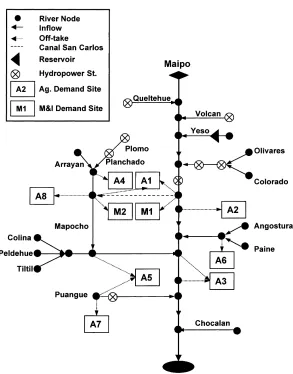
Fig. 1. The Maipo river basin network.
An existing hydrologic model, successfully applied to the Amu Darya and Syr Darya river basins in Central Asia, has been adapted to the Chilean context (McKin-ney and Cai, 1997). In addition, a prototype economic optimization model has been developed in order to es-timate economic returns to water use. Although the model has been developed as an optimization model, simulation components have been included to better solve the complex optimization problem. Hydrologic flow and salinity balance and tranport are simulated endogenously within the optimization model and an external crop–water simulation model is used to esti-mate the crop yield function, with water, salinity and irrigation technology as variables.
extension to the irrigated crop fields at each irriga-tion demand site. Water demand and water supply are then integrated into an endogenous system and balanced based on the economic objective of maxi-mizing benefits from water use, including irrigation, hydropower, and M&I benefits. Both water quantity and water quality in terms of salinity are simulated in the model. The salt concentration in the return flow from irrigated areas is explicitly calculated in the model. This allows the endogenous considera-tion of this externality with respect to upstream and downstream irrigation districts. The model includes all the essential relationships of these components in a 1-year time horizon with a monthly time step.
3.2. Model components
Thematically, the modeling framework includes three components: (1) hydrologic components, in-cluding the water and salt balance in reservoirs, river reaches and aquifers within the river basin; (2) water use components, including water for irrigation and M&I water uses; and (3) economic components, in-cluding the calculation of benefits from irrigation, hydropower, and M&I demand sites.
Hydrologic relations and processes are based on the flow network, which is an abstracted representation of the spatial relationships between the physical entities in the basin. The major hydrologic relations/processes include: flow transport and balance from river out-lets/reservoirs to crop fields or M&I demand sites; salt transport and balance from river outlets/reservoirs to irrigated crop fields; return flows from irrigated and urban areas; interaction between surface and groundwater; evapotranspiration in irrigated areas, and hydropower generation as well as physical bounds on storage, flows, diversions and salt concentrations. The mathematical expressions for these relations, as well as the calculation of deep percolation, return flow from agricultural and M&I demand sites, and the interaction between surface and groundwater can be found in Rosegrant et al. (1999). It is assumed that the water supply starts from rivers and reservoirs. Effective rainfall is calculated outside of the model, and included into the model as a constant parameter.
The agronomic relations involved in the simulation model are adapted from Dinar and Letey (1996), (see also Letey and Dinar, 1986, and Dinar et al., 1991).
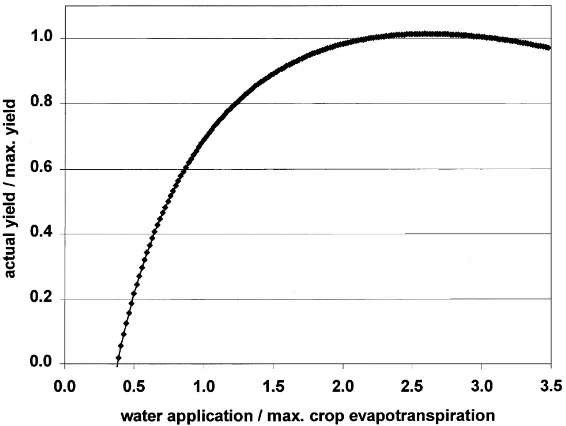
A curve–linear relationship is assumed between crop yield and seasonally applied non-saline water. Crop yield is simulated under given water application, irri-gation technology (the Christiensen Uniformity Coef-ficient or CUC), and irrigation water salinity. Based on these simulation results, a regression function of crop yield with water application, irrigation uniformity, and salinity was derived through the estimation of the parameters a0–a2and b0–b8in Eq. (1). The function, with specific parameters that have been estimated for all crops in the model, is directly used in the opti-mization model to calculate crop yields with varying water application, salt concentration, and CUC.
The crop yield function is specified as follows:
Ya=Ymax[a0+a1(wi/Emax)+a2ln(wi/Emax)] (1) where
a0=b0+b1u+b2c, a1=b3+b4u+b5c, a2=b6+b7u+b8c
and where Ya is the crop yield (metric tons (mt)/ha), Ymaxthe maximum attainable yield (mt/ha), a0, a1, a2 are regression coefficients, b0–b8are regression coef-ficients,wi is infiltrated water (mm), Emaxthe maxi-mum evapotranspiration (mm), c the salt concentration in water application (dS/m), and u the Christiensen Uniformity Coefficient (CUC).
Uniformity (CUC) is used as a surrogate for both irrigation technology and irrigation management ac-tivities. The CUC value varies from approximately 50 for flood irrigation, to 70 for furrow irrigation, 80 for sprinklers, and 90 for drip irrigation, and also varies with management activities. By including explicit representation of technology, the choice of water application technology can be determined endoge-nously. The profit from agricultural demand sites is equal to crop revenue minus fixed crop cost, irriga-tion technology improvement cost, and water supply cost. The function for profits from irrigation (VA) at demand site dm, is specified as follows:
M.W. Rosegrant et al. / Agricultural Economics 24 (2000) 33–46 37
Fig. 2. Crop yield function, crop yield (wheat) vs. water application (CUC=70, Salinity=0.7 dS/m).
in which A is harvested area (ha), cp the crop type, p the crop price (US$/mt), fc the fixed crop cost (US$/ha), tc = k010(−k1u) the technology cost (US$/ha) (formulation following Dinar and Letey (1996) — higher CUC values are associated with greater capital cost for irrigation and/or management costs), wp the water price (US$/m3),wthe water de-livered to demand sites (m3), k0 the intercept of the technology cost function, and k1 cost coefficient per unit of u.
A typical crop yield function for wheat in the Maipo river basin is shown in Fig. 2. The function drives the seasonal water allocation among crops, but is not able to distribute the diverted water among crop growth stages according to the water demanded by each stage. In order to achieve consistency with the water balance in the hydrologic system — to fill the gap between the agronomy and hydrology in the optimization model — an empirical yield–evapotranspiration relationship given by Doorenbos and Kassam (1979) has been used to account for the stage effect. This relationship was applied by including a penalty term into the objective function, based on the maximum stage yield deficit (see below for the specification of the penalty term). The penalty drives the water application according to the water demands in crop growth stages.
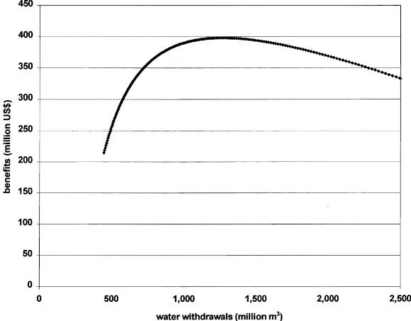
The net benefit function for M&I water use is de-rived from an inverse demand function for water. Net benefit is calculated as water use benefit minus water supply cost.
VM(w)=w0p0/(1+α)(w/w0)α+2α+1−wwp (3)
where VM is the benefit from M&I water use (US$), w0the maximum water withdrawal (m3), p0the will-ingness to pay for additional water at full use (US$), α is 1/e, e the price elasticity of demand (currently −0.45).
Fig. 3. Relationship between water withdrawals and M&I benefits.
withdrawals and benefits for the M&I net benefit function.
Benefits from power generation are relatively small in the Maipo Basin compared to off-stream water uses. The profit from power generation (VP) at a power station, pwst, is calculated as
VP(pwst)=X pd
power(pwst,pd)
×[pprice(pwst)−pcost(pwst)] (4)
where power is the power production, for each power station and period (kW h), which is a function of wa-ter flow for runoff stations, and of wawa-ter release and reservoir head for stations with dams, as well as hy-dropower generating capacity and efficiency; pprice is the price of power production for each power station (US$/kWh); and pcost is the cost of power production, for each power station (US$/kW h).
The model also includes a series of institutional rules, including minimum required water supply to a demand site, minimum and maximum crop produc-tion, flow requirement through a river reach for en-vironmental and ecological purposes, and maximum allowed salinity in the water system. The objective is
to maximize economic profit from water supply for irrigation, M&I water use, and hydroelectric power generation, subject to institutional, physical, and other constraints. The objective function is specified as follows:
Max Obj= X irr−dem
VA(dm)+ X mun−dem
VM(dm)
+X
pwst
VP(pwst)−wgt penalty (5)
where wgt is the weight for the penalty, and penalty is defined as
penalty=X dem
X
cp
pm(cp)×cpprice(cp)
×(mdft(dem,cp)−adft(dem,cp)) (6)
where, over all demand sites and crops, pm is max-imum crop production (mt), cpprice the crop selling price (US$/mt), mdft the maximum stage deficit within a crop growth season, and adft the average stage deficit within a crop growth season.
with
dft=ky
1− Ea Emax
M.W. Rosegrant et al. / Agricultural Economics 24 (2000) 33–46 39 where dft is the stage deficit, ky the yield response
factor, and Ea the actual evapotranspiration (mm), as defined in Doorenbos and Kassam (1979).
3.3. Model solution
The model has been coded in the modeling language of the General Algebraic Modeling System (GAMS) (Brooke et al., 1988), a high-level modeling system for mathematical programming problems. Since the model is highly non-linear and includes a large num-ber of variables and equations, it is solved in two steps. In the first step, the salinity variable is fixed. The so-lution of this model is used for the initial values of the variables in the second model with variable salt concentration (see Cai, 1999).
4. Results and policy analysis
The focus of the modeling in this paper is on the agriculture sector and to a lesser extent on the non-agricultural water sectors.
4.1. Basin-optimizing solution (‘baseline’)
Assumptions in the basoptimizing solution in-clude a water price in M&I demand sites of US$ 0.1 per m3 and in agricultural demand sites of US$ 0.04 per m3. Crop technology is fixed at CUC equal
Table 1
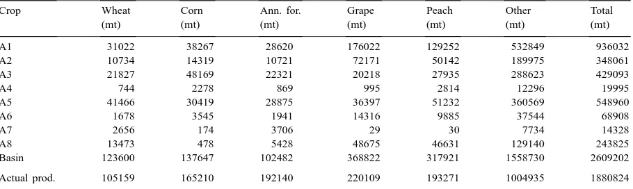
Crop production in the basin, basin-optimizing result and actual dataa
Crop Wheat Corn Ann. for. Grape Peach Other Total
(mt) (mt) (mt) (mt) (mt) (mt) (mt)
A1 31022 38267 28620 176022 129252 532849 936032
A2 10734 14319 10721 72171 50142 189975 348061
A3 21827 48169 22321 20218 27935 288623 429093
A4 744 2278 869 995 2814 12296 19995
A5 41466 30419 28875 36397 51232 360569 548960
A6 1678 3545 1941 14316 9885 37544 68908
A7 2656 174 3706 29 30 7734 14328
A8 13473 478 5428 48675 46631 129140 243825
Basin 123600 137647 102482 368822 317921 1558730 2609202
Actual prod. 105159 165210 192140 220109 193271 1004935 1880824
aActual production is average for 1994–1996. As crop diversity in the basin is extremely high, some crops are averages of aggregate production of similar crops. Peach, for example, includes almond, apricot, cherry, nectarines, peach, and plum. Source of actual production data: Donoso, 1997.
to 70. Moreover, it is assumed that 15% of the in-flow is reserved for environmental (instream) uses. The source salinity is 0.3 g/l. No water right is set up and water withdrawals to demand sites depend on their respective demands with the objective of maximizing basin benefits.
Table 2
Harvested area, basin-optimizing resulta
Crop Wheat Corn Annual forage Grape Peach Other Total
(ha) (ha) (ha) (ha) (ha) (ha) (ha)
A1 5607 4196 2529 9264 6463 20271 48329
A2 1925 1574 936 3798 2527 7035 17795
A3 3899 5219 1925 1064 1401 12620 26128
A4 135 248 76 52 141 505 1157
A5 7446 3344 2521 1916 2574 15840 33642
A6 302 384 170 753 494 1367 3471
A7 482 19 325 2 2 397 1227
A8 2440 53 481 2562 2346 6377 14258
Basin 22235 15037 8963 19412 15947 64412 146007
Model/actual 1.0 0.8 0.6 1.5 1.5 1.3 1.1
aSource of actual harvested area: Donoso, 1997.
estimated at 3817 million m3, 86% of the total inflows of 4445 million m3. Water withdrawals are lowest in the months of June and July, as only perennial crops are present during this time. An apparent excess use of surface water — withdrawals exceed source flows — during the months of January–March and November–December can be explained with the high level of return flows that are being reused during these months. Total return flows amount to 872 million m3 or 20% of total inflows. Actual crop evapotranspira-tion is estimated at 954 million m3, 99.7% of the total potential crop evapotranspiration of 956 million m3. This value compares well with the data estimated in Donoso (1997) of 972 million m3. According to the model results, total agricultural water withdrawals
Table 3
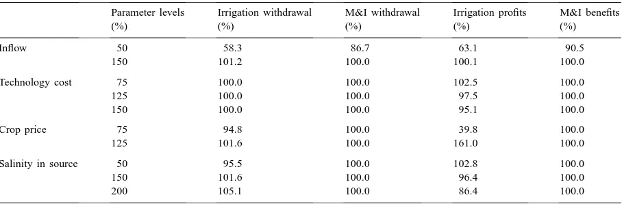
Sensitivity analysis, various parametersa
Parameter levels Irrigation withdrawal M&I withdrawal Irrigation profits M&I benefits
(%) (%) (%) (%) (%)
Inflow 50 58.3 86.7 63.1 90.5
150 101.2 100.0 100.1 100.0
Technology cost 75 100.0 100.0 102.5 100.0
125 100.0 100.0 97.5 100.0
150 100.0 100.0 95.1 100.0
Crop price 75 94.8 100.0 39.8 100.0
125 101.6 100.0 161.0 100.0
Salinity in source 50 95.5 100.0 102.8 100.0
150 101.6 100.0 96.4 100.0
200 105.1 100.0 86.4 100.0
aSensitivity analyses, except for the inflow scenarios, were carried out based on normal flow. All percentages are relative to the baseline. amount to 2360 million m3, which again is close to the 2107 million m3estimated in Donoso (1997). The difference can be explained, in part, by the different irrigation efficiencies. The overall efficiency estimated by local experts is about 45%, whereas the efficiency according to model results is 40.4%.
4.2. Sensitivity analysis
M.W. Rosegrant et al. / Agricultural Economics 24 (2000) 33–46 41 Table 4
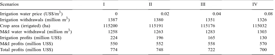
Sensitivity analysis for irrigation water price at 50% of normal inflow
Scenarios I II III IV
Irrigation water price (US$/m3) 0 0.02 0.04 0.08
Irrigation withdrawals (million m3) 1387 1380 1351 1326
Crop area (irrigated) (ha) 115200 115191 115176 115032
M&I water withdrawal (million m3) 1258 1263 1283 1303
Irrigation profits (million US$) 224 196 165 130
M&I profits (million US$) 550 552 558 570
Total profits (million US$) 774 748 722 700
changing range of technology cost, crop price, and source salinity under conditions of normal flow. This is because, at normal inflows, the M&I demand sites can withdraw up to their benefit-maximizing level within the varying range of those parameters. However, M&I withdrawals and benefits do vary in the dry-year case (see Table 4).
With a reduction of normal inflows by half, wa-ter withdrawals and benefits for both agricultural and M&I demand sites decline sharply. Agricultural prof-its decrease by 37% and M&I benefprof-its decline by 9% compared to normal inflows. Moreover, water with-drawals plunge by 42% for irrigation and by 13% in M&I demand sites. Thus, in the case of drought, the agriculture sector is much more affected. Agricultural water withdrawals are not sensitive to the cost of ir-rigation technology and profits from irir-rigation vary only slightly with changes in technology cost. Pro-portional changes over all crop prices in the range of ±25% have only small effects on irrigation water with-drawals. However, farmer incomes from irrigation are significantly affected. With a reduction of crop prices by 25%, irrigation water withdrawals decline by 5%, whereas profits from irrigation drop by 60%.
A doubling of the source salinity leads to an in-crease in irrigation water withdrawals for salt leaching by 5%. Increased salt leaching reduces profits from irrigation by 14%. Moreover, changes in the salinity level influence crop patterns, with a decline in the har-vested area of crops with lower salt tolerance. With doubled source salinity, the area planted to maize de-clines from 10 to 8% of total area planted whereas the area planted with wheat — a more salt tolerant crop — increases from 15 to 18%.
Table 4 shows the effects of changes in the wa-ter price for agriculture on wawa-ter withdrawals and
incomes in the irrigation and M&I sectors for a drought-year case (50% of normal inflows). With an increase in the water price for irrigation from zero to US$ 0.08 per m3, water withdrawals for agriculture decline by 5%, from 1387 to 1326 million m3. How-ever, changes in the water price barely affect the crop area. Irrigated area is maintained because farmers shift on the margin to more water efficient crops and reduce water use per hectare. Although both water withdrawals and irrigated crop area barely change with varying water prices, farmer incomes can drop drastically under this ‘administrative price scenario’: by 42% from US$ 224 million to US$ 130 million with increasing prices. M&I benefits, on the other hand, increase steadily with continuing water price increases in agriculture, from US$ 550 million to US$ 570 million and M&I water withdrawals increase by 3.6%. With water prices already quite high (higher than what most farmers in the United States pay), further price increases are a blunt instrument for in-fluencing water demand. Under these circumstances, water markets that allow farmers to retain the income from sales of water may be preferable.
4.3. Economic analysis of water trading
There are two fundamental strategies for dealing with water scarcity in river basins, supply manage-ment and demand managemanage-ment; the former involves activities to locate, develop, and exploit new sources of water, and the latter addresses the incentives and mechanisms that promote water conservation and efficient use of water.
water rights. The empirical evidence shows that farm-ers are price responsive in their use of irrigation water (Rosegrant et al., 1995; Gardner, 1983). The choice between administered prices and markets should be largely a function of which system has the lowest administrative and transaction costs (TC). Markets in tradable water rights can reduce information costs; in-crease farmer acceptance and participation; empower water users; and provide security and incentives for investment and for internalizing the external costs of water uses. Market allocation can provide flexibility in response to water demands, permitting the selling and purchasing of water across sectors, across dis-tricts, and across time by opening opportunities for exchange where they are needed. The outcomes of the exchange process reflect the water scarcity condition in the area with water flowing to the uses where its marginal value is highest (Rosegrant and Binswanger, 1994; Rosegrant, 1997). Markets also provide the foundation for water leasing and option contracts, which can quickly mitigate acute, short-term urban water shortages while maintaining the agricultural production base (Michelsen and Young, 1993). Estab-lishment of markets in tradable property rights does not imply free markets in water. Rather, the system would be one of managed trade, with institutions in place to protect against third-party effects and po-tential negative environmental effects that are not eliminated by the change in incentives. Tradable wa-ter rights could lead to massive transfers of wawa-ter to urban and industrial centers. Therefore, farmers need to be protected by adequate institutions and organiza-tions. The Chilean Water Law of 1981 established the basic characteristics of property rights over water as a proportional share over a variable flow or quantity. Changes in the allocation of water within and be-tween sectors are realized through markets in tradable water rights (for details, see Gazmuri Schleyer and Rosegrant, 1996; Hearne and Easter, 1995).
The integrated economic–hydrologic river basin model allows for a fairly realistic representation and analysis of water markets. Water trading in the basin is constrained by the hydrologic balance in the river basin network; water is traded taking account of the physical and technical constraints of the various de-mand sites, reflecting their relative profitability in trading prices; water trades reflect the relative sea-sonal water scarcity in the basin that is influenced
by both basin inflows and the cropping pattern in agricultural demand sites (whereas the M&I water demands are more stable); and negative externalities, like increased salinity in downstream reaches due to incremental irrigation water withdrawals upstream, are endogenous to the model framework.
4.3.1. Model formulation for water trading
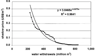
To extend the model to water trading analysis, in a first step, a shadow price — water withdrawal re-lationship is determined for each demand site. For this, the model is run separately for each demand site with varying water withdrawals as inputs and shadow prices or marginal values as output derived from the water balance equations (each irrigation demand site includes a water balance equation for each of up to 15 crops). These shadow prices are then averaged over all crops to obtain one shadow price for each water sup-ply level for each demand site. Based on these input and output values a regression function is estimated for the shadow price — water withdrawal relationship for each demand site. Fig. 4 shows the model results and the regression relationship between shadow price and water withdrawals for an agricultural demand site. Water rights are allocated proportionally to total in-flows based on historical withdrawals for M&I areas and on the harvested (irrigated) area for agricultural demand sites. Thus, with reduced inflows, the realized volumes of the water rights change without changes in the rights structure. The water right refers to surface water only. To determine the lower bound for profits from water trade by demand site (it is assumed that no demand site can lose from trading), the model is solved for the case of water rights without trading. Finally, the regression relationships of shadow price
M.W. Rosegrant et al. / Agricultural Economics 24 (2000) 33–46 43 versus water withdrawal for all agricultural and M&I
demand sites, the water rights, and other water trad-ing related constraints (see Rosegrant et al., 1999) are added to the basin model. It is assumed that the trad-ing price for each demand site is equal to its shadow price for water. This model is then solved to determine the water trading price, wtp, and the volume of water bought and sold by demand site.
Trade is allowed on a monthly basis and through-out the basin and TC are incurred by both buyer and seller (US$ 0.04 per m3). Up to 4 months of the real-ized monthly water right can be traded as the monthly balances had been found as too tight of a constraint on water supply for crop growth.
4.3.2. Water trading analysis
Three scenarios are compared to assess the im-pact of water trading: a baseline with omniscient
Table 5
Scenario analysis: basin-optimizing solution, water rights without trade, and water rights trading
Site Withdrawals Water right Net trade Net profits ‘Gains’b Shadow price of water
BO WR WRTa WR&WRT WRT BO WR WRT WRT BO WR WRT
(million m3) (million US$) (US$/m3)
Case A: 100% of normal inflow
A1 696 617 610 867 13 120 117 118 1 0.044 0.128 0.132
A2 266 243 234 341 8 46 45 45 1 0.044 0.111 0.123
A3 371 391 349 547 70 47 49 52 2 0.046 0.075 0.119
A4 16 15 14 21 3 2 2 3 0 0.045 0.083 0.111
A5 506 502 444 704 147 65 67 71 5 0.051 0.091 0.138
A6 54 46 45 64 1 9 8 8 0 0.045 0.134 0.147
A7 15 17 14 25 10 2 2 2 1 0.072 0.040 0.099
A8 206 154 153 216 1 37 31 31 0 0.044 0.189 0.177
M1 991 678 841 678 −163 417 293 353 60 0.019 0.975 0.415
M2 460 315 404 315 −90 193 135 166 32 0.019 1.014 0.383
Total 3581 2977 3108 3778 0 939 749 850 101
Case B: 60% of normal inflow
A1 514 479 432 522 47 95 89 99 10 0.097 0.134 0.232
A2 222 188 166 205 90 40 36 52 17 0.102 0.230 0.221
A3 305 303 279 329 23 41 41 43 3 0.078 0.168 0.194
A4 7 11 10 13 2 1 1 2 1 0.096 0.100 0.195
A5 395 391 350 423 112 56 55 70 16 0.110 0.111 0.192
A6 43 34 33 38 2 8 7 7 1 0.077 0.225 0.224
A7 11 11 11 15 2 1 1 2 1 0.127 0.059 0.146
A8 142 120 102 130 18 27 23 25 2 0.098 0.259 0.259
M1 974 518 713 408 −195 413 102 266 164 0.056 1.439 0.789
M2 453 240 342 189 −101 192 34 129 94 0.056 1.720 0.735
Total 3067 2296 2437 2272 0 874 389 696 307
aThese withdrawals are net of water traded. bGains are gains from trade.
decision-maker optimizing benefits for the entire basin (BO); water rights with no trading permitted (WR), and water rights with trading (WRT). The salinity variable is fixed for all three water trading scenarios. The results compare two cases for each of these three scenarios: hydrologic level at 100% of the normal inflow and at 60% of the normal inflow (Table 5). In addition, three TC scenarios are analyzed based on normal inflow (Table 6). The description of results will concentrate on the drought-year scenario (case B, 60% of normal inflow), as the benefits vary more clearly by economic instrument employed.
Table 6
Transaction cost scenarios (case A) Transaction
0.00 3119 278 871 122 0.1808
0.04 3108 264 850 101 0.1844
0.10 3075 236 822 73 0.4127
0.20 3051 138 755 6 1.2680
the basin and institutional requirements. Water with-drawals decline substantially in the WR case, relative to BO, when withdrawals are limited to the respective water right and trading is not allowed. Agricultural withdrawals are often actually below the actual water right, because dry-season flows are inadequate to ful-fill all crop water requirements. Another reason is that, in about half of the months, only perennial crops are grown, and thus withdrawals are far below the allotted flow.
When water can be traded, irrigation withdrawals actually decline further, albeit not very much. Ir-rigation withdrawals decline because the irIr-rigation districts sell part of their water right to the M&I de-mand sites, thereby reaping substantial profits. In the dry-year case, a total water volume of 296 million m3 is traded, about 11% of total dry-year inflows. In the case of normal inflows, 264 million m3 of water is traded, about 6% of total inflow. M&I areas are the main buyers in both cases, purchasing virtually all the water offered by the irrigation districts. All irrigation districts are net sellers of water over the course of the year. Under the drought-year case, only district A8 purchases 0.2 million m3 of water to maintain its cropping pattern that features the largest share of higher-valued, perennial crops (grapes, peach, among others, see Table 2). In the case of normal inflows, on the other hand, the marginal value of water is much lower, and two agricultural demand sites, A6 and A8, purchase water (0.2 million m3 and 10.8 million m3, respectively) to supplement their crop production in some months; however, overall both districts are net sellers of water.
As the WR system does not allow the transfer of water to more beneficial uses, benefits from water uses are significantly reduced by locking the resource into relatively low valued uses during shortages. As
a result, total net benefits are less than one-half of the optimizing solution (US$ 389 million compared with US$ 874 million). By permitting trading, wa-ter moves from less productive agricultural uses into higher-valued urban water uses while at the same time benefiting farm incomes. Total benefits in the M&I demand sites almost triple, compared to the WR case, but gains are also significant for the irrigation districts and each district can increase net profits, by between 6 and 62%, depending on their respective physical and other characteristics. Total net profits of the sector increase by about 20%, from US$ 253 mil-lion to US$ 301 milmil-lion. In irrigation districts A1–A5 and A7, total net profits under the WRT scenario are even higher than for the basin-optimizing case. This is due to the higher value of the scarcer water and the resulting benefits from trade and does not occur in case A with normal inflow levels.
Moreover, net profits from crop production decline only slightly with trading: from US$ 253 million to US$ 244 million. Total crop production also barely declines, from 1.866 million mt to 1.729 million mt. In addition, the proportion of higher-value peren-nial crops increases substantially from the WR to the WRT scenarios, from 14 to 19% for grapes and from 13 to 16% for peach, for example. These results not only show the advantages of the water market approach compared to the WR case, but also to the administrative price scenario presented in the sensi-tivity analysis, in which water is also reallocated from agricultural to non-agricultural uses, but at a punitive cost to agricultural incomes.
M.W. Rosegrant et al. / Agricultural Economics 24 (2000) 33–46 45 because no monitoring/transaction costs are charged
for the omniscient decision-maker when in fact the cost would likely be very high.
For the water trading scenario, it is currently as-sumed that both buyer and seller contribute equally to TC (US$ 0.04 per m3). Three TC scenarios were run in addition to this base trading scenario: zero TC, US$ 0.1 per m3, and US$ 0.2 per m3. The results are shown in Table 6. As can be expected, water withdrawals decline with increasing TC, and the volume of water traded plunges by more than half, from 278 million m3 for the case without TC to 138 million m3 for the case with TC of US$ 0.2 per m3. This is due, in part, to the fact that the TC are quite high relative to the shadow prices for water, which range from US$ 0.18 to 1.27 per m3. Total net benefits decline substantially, from US$ 871 million at zero TC to US$ 755 million at TC of US$ 0.2 per m3; gains from trade also drop sharply, from US$ 122 million to only US$ 6 million, respectively. Thus, making trading more efficient (re-ducing TC) has significant benefits, increasing both the volume and the benefits from trade.
5. Conclusions
This paper presents a prototype river basin model that includes essential hydrologic, agronomic and economic relationships, and reflects the inter-relationships of water and salinity, food production, economic welfare, and environmental consequences. The model is applied to the Maipo river basin in Chile, but due to its generic form and structure can be applied to other basins.
The model results show the benefits of water rights trading with water moving into higher valued cultural (and M&I) uses. Net profits in irrigated agri-culture increase substantially compared to the case of proportional use rights for demand sites. Moreover, agricultural production does not decline significantly. Net benefits for irrigation districts can be even higher than for the basin-optimizing case, as farmers reap substantial benefits from selling their unused water rights to M&I areas during the months with little or no crop production. Finally, making trading more ef-ficient, that is, reducing transaction costs, has signi-ficant benefits, increasing both the amount of trading and the benefits from trade.
Although these preliminary results show the effec-tiveness of the model for policy analysis and water allocation in the river basin, additional research is needed. During a second research phase, the agricul-tural production functions will be extended to include inputs in addition to land, water, and irrigation tech-nology, such as agricultural chemicals and labor. In addition, the urban water demand functions will be re-estimated based on empirical data and disaggre-gated into household and industrial water demands. Moreover, the power generation will be calibrated to local parameters. Based on this extension, more comprehensive policy analysis will be carried out. Existing institutions regarding water rights, priority allocations, and additional institutional realities will be better represented based on local data. Finally, di-rect cooperation will be established with the relevant government authorities and water user associations in the basin, with the goal of institutionalizing the model as a decision support system for basin water policy.
Acknowledgements
Senior authorship is shared. Generous support has been received from the Inter-American Development Bank, the USAID-CGIAR University Partnership Funds, and the System-Wide Initiative on Water Management (SWIM) of the International Water Management Institute.
References
Anton, D.J., 1993. Thirsty cities: urban environments and water supply in Latin America. International Development Research Centre, Ottawa, Ontario.
Bolelli, M.J., 1997. EMOS y su relación con la cuenca: Demanda de recursos h´ıdricos y manejo de aguas servidas. In: Anguita, P., Floto, E. (Eds.), Gestión del recurso h´ıdrico, Proceedings of the International Workshop organized by the DGA and the Dirección de Riego of the Ministerio de Obras Públicas and the FAO, 2–5 December 1996, Santiago de Chile.
Brooke, A., Kendrick, D., Meeraus, A., 1988. GAMS: A User’s Guide. Scientific Press, San Francisco, California.
Cai, X., 1999. A modeling framework for sustainable water resources management, Ph.D. Dissertation, The University of Texas, Austin.
UN/ECLAC (Ed.), Water management and environment in Latin America. Pergamon Press, New York.
Dinar, A., Letey, J., 1996. Modeling economic management and policy issues of water in irrigated agriculture. Praeger, Westport, Connecticut.
Dinar, A., Hatchett, S.A., Loehman, E.T., 1991. Modeling regional irrigation decisions and drainage pollution control. Natural Resour. Model. 5, 191–211.
Donoso, G., 1997. Data collection to operationalize a prototype river basin model of water allocation: Maipo-Mapocho basin. Mimeo.
Doorenbos, J., Kassam, A.H., 1979. Yield response to water. FAO Irrigation and Drainage Paper No. 33. FAO, Rome.
Gardner, B.D., 1983. Water pricing and rent seeking in California agriculture. In: Anderson, T.L. (Ed.), Water Rights, Scarce Resource Allocation, Bureaucracy, and the Environment. Ballinger, Cambridge, MA.
Gazmuri Schleyer, R., Rosegrant, M.W., 1996. Chilean water policy: the role of water rights, institutions and markets. Int. J. Water Resour. Develop. 12, 33–48.
Hearne, R.R., 1998. Institutional and organizational arrangements for water markets in Chile. In: Easter, K.W., Rosegrant, M.W., Dinar, A. (Eds.), Markets for Water: Potential and Performance. Kluwer Academic Publishers, Boston.
Hearne, R.R., Easter, K.W., 1995. Water allocation and water markets: an analysis of gains-from-trade in Chile. World Bank Technical Paper No. 315, Washington, DC, World Bank.
Letey, J., Dinar, A., 1986. Simulated crop-water production functions for several crops when irrigated with saline waters. Hilgardia 54, 1–32.
McKinney, D.C., Cai, X., 1997. Multiobjective water resources allocation model for the Naryn-Syrdarya Cascade. Technical Report. US Agency for International Development, Environmental Policies and Technology (EPT) Project, Almaty, Kazakstan.
Michelsen, A.M., Young, R.A., 1993. Optioning agricultural water rights for urban water supplies during drought. Am. J. Agri. Econ. 75, 1010–1020.
Randall, A., 1981. Property entitlements and pricing policies for a maturing water economy. Austr. J. Agri. Econ. 25, 192– 220.
Rosegrant, M.W., et al. 1999. Report for the IDB on the integrated economic–hydrologic water modeling at the basin scale: the Maipo river basin in Chile. IFPRI, Washington DC.
Rosegrant, M.W., 1997. Water resources in the twenty-first century: challenges and implications for action. Food, Agriculture, and the Environment Discussion Paper No. 20. IFPRI, Washington, DC.
Rosegrant, M.W., Gazmuri Schleyer, R., Yadav, S., 1995. Water policy for efficient agricultural diversification: market-based approaches. Food Policy 18, 203–223.