MODELING SPATIAL DISTRIBUTION OF A RARE AND ENDANGERED PLANT
SPECIES (
Brainea insignis
) IN CENTRAL TAIWAN
Wen-Chiao Wanga, Nan-Jang Lob, Wei-I Changc, Kai-Yi Huangd
a
Graduate student, Dept. of Forestry, Chung-Hsing University, Taiwan E-mail: [email protected] b
Specialist, EPMO, Chung-Hsing University, Taiwan E-mail: [email protected] c
Director, HsinChu FDO, Forest Bureau, Council of Agriculture, Taiwan E-mail: [email protected] d*
Professor, same as with author-a E-mail: [email protected] (corresponding author) 250 Kuo-Kuang Road, Taichung, Taiwan 402, Tel: +886-4-22854663; Fax: +886-4-22854663
Commissions: VII/4 methods for land cover classification
KEY WORDS: Forestry, Ecology, Modeling, Prediction, Algorithms, Pattern, Performance, Accuracy.
ABSTRACT:
With an increase in the rate of species extinction, we should choose right methods that are sustainable on the basis of appropriate science and human needs to conserve ecosystems and rare species. Species distribution modeling (SDM) uses 3S technology and statistics and becomes increasingly important in ecology. Brainea insignis (cycad-fern, CF) has been categorized a rare, endangered plant species, and thus was chosen as a target for the study. Five sampling schemes were created with different combinations of CF samples collected from three sites in Huisun forest station and one site, 10 km farther north from Huisun. Four models, MAXENT, GARP, generalized linear models (GLM), and discriminant analysis (DA), were developed based on topographic variables, and were evaluated by five sampling schemes. The accuracy of MAXENT was the highest, followed by GLM and GARP, and DA was the lowest. More importantly, they can identify the potential habitat less than 10% of the study area in the first round of SDM, thereby prioritizing either the field-survey area where microclimatic, edaphic or biotic data can be collected for refining predictions of potential habitat in the later rounds of SDM or search areas for new population discovery. However, it was shown unlikely to extend spatial patterns of CFs from one area to another with a big separation or to a larger area by predictive models merely based on topographic variables. Follow-up studies will attempt to incorporate proxy indicators that can be extracted from hyperspectral images or LIDAR DEM and substitute for direct parameters to make predictive models applicable on a broader scale.
1. INTRODUCTION
Biodiversity is very important for humans and all other species on the Earth. Without the diversity of species, ecosystems are more fragile to natural disasters and climatic change. With an increase in the rate of species extinction, we must conserve ecosystems and rare species by choosing right methods that are sustainable on the basis of appropriate science and human needs. Forest resources in Taiwan are very abundant, but environmental carrying capacity of the island is vulnerable, thus when using them we must think of conservation at the same time.
Species distribution modeling (SDM) could apply in conservation and protection rare species, ecology, epidemiology, disaster and management in forestry (Pearson et al., 2007; Asner et al., 2008; Cayuela et al., 2009). SDM needs to utilize the combination of 3S technology and statistics, and has become increasingly important in ecology (Côté and Reynolds, 2002; Guisan and Thuiller, 2005). Nowadays a variety of statistical methods have been used to model ecological niches and predict the geographical distributions of species, such as BIOCLIM, maximum entropy (MAXENT), DOMAIN, genetic algorithm for rule-set prediction (GARP), generalized linear models (GLM), generalized additive model (GAM) and discriminant analysis (DA) (Elith et. al., 2006; Hernandez et al., 2006; Guisan et al., 2007; Peterson et al., 2007; Wisz et al., 2008; Ke et al., 2010).
SDM is based on the environmental conditions of known sites to predict unknown area, and also to identify the relationship between the species and environment. The distribution pattern of natural vegetation is associated with four types of environmental factors, including climatic, physiographic, edaphic, and biotic factors (Su, 1987). For SDM, it is
desirable to predict a species distribution on the basis of ecological (direct) parameters (i.e. climate, soil, and biotic factor) that are to be the causal, driving forces for its distribution. Data for such direct parameters, however, are generally difficult or expensive to measure, soil data are even more difficult to derive, and they tend to be less accurate than pure topographic characteristics (Guisan and Zimmermann, 2000). Moreover, biotic factor is extremely difficult to estimate due to the fine spatiotemporal resolution and potentially complex nature of biotic dimensions (Barve et. al., 2011). On the other hand, indirect parameters (e.g. topographic variables: elevation, slope, aspect) are most easily measured by remote sensing and are often used because of their good correlation with observed species patterns (Guisan and Zimmermann, 2000). Hence, SDM should be run on an iterative basis with topographic data in initial rounds and climatic data, soil data, or biotic data, when available, in later rounds since not all the data needed by SDM for the four types of factors aforementioned are readily available at one time.
terms of accuracy and implementation efficiency and determined the optimum for predicting the habitat of a rare plant. The predictive outcome from SDM would be used to prioritize field-survey areas for collecting fine resolution microclimatic, edaphic or biotic data for refining predictions of potential habitat in the later rounds of SDM or search areas for new population discovery.
2. STUDY AREA
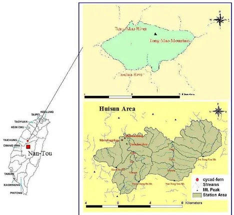
The study area consists of two parts, one part is Huisun Experimental Forest Station (HEFS), and the other is Tong-Mao Mountain, as shown in Figure 1. HEFS is in central Taiwan, and situated within 24◦2´–24◦5´ N latitude and
121◦3´–121◦7´ E longitude. This station is the property of Chung-Hsing University, and has a total area of 7, 477 ha. This station ranges in elevation from 454 m to 3, 419 m, and its climate is temperate and humid. Hence, this area has nourished about 1,100 plant species and is a representative forest in central Taiwan. This study took the samples from Sihwufongshan (Pine-breeze Mountain), Duhchuanling (Cuckoo Ridge) and Kuandaushan (Big-knife Mountain) trail in Huisun, Sihwufongshan elevation from 680 m to 840 m, the highest elevation of Duhchuanling approximately 810 m, and Kuandaushan elevation approximately 760 m. According to the climate record of this study area, the annual mean temperature is 21.0℃; the monthly mean temperature highest is 30.6℃ in July, lowest is 20.5℃in January; mean annual precipitation 2453.5 mm, the average relative humidity is 85%. Tong-Mao Mountain is situated at geographic coordinate 24°11'N latitude and 120°57' E longitude, near the Ta-chia River and Tong-Mao River, 10 km farther north from Huisun area. The elevation of Tong-Mao Mountain rises to 1690 m above sea level. According to the climate record of forest district office website, the annual mean temperature is 22.6℃; mean temperature highest is 29℃ in July, lowest is 15℃ in January; mean annual precipitation 2580 mm. The mountain has rich ecological resources cycad-fern (CF), Blechnaceae
family, is only found in mountains in central Taiwan, such as Huisun and Tong-Mao Mountain areas, and Huisun is the main habitat. Because of its limited ecological range, cycad-fern has been categorized as one of the rare, endangered species (Lu
et al, 1986).
Figure 1 Location map of the study area.
3. MATERIALS AND METHODS
3.1 Data Collection
We collected digital elevation model (DEM) with grid size 5 × 5 m, orthophoto base maps (1:10,000), and nine-date SPOT images (SPOT Image Copyright 2004 and 2005, CNES). In situ data (cycad-fern samples) were also acquired by using a GPS linked with an expandable antenna rod of 5m in length and a laser range finder, the error was usually below one meter after post-processing differential correction. Two-date SPOT images (07/10/2004 and 11/11/2005) were chosen because they have the best quality with the least amount of clouds among the nine-date SPOT images.
3.2 Data Processing
Slope and aspect data layers were generated from 5 × 5 m DEM. The ridges and valleys in the study area were used together with DEM to generate terrain position layer. The main ridges and valleys were directly interpreted from the contour lines shown on the orthophoto base maps; these lines were then digitized to establish the data layer by using ARC/INFO software for later use. The relative position (Pij) of the test cell in the terrain is expressed as follows:
Pij=PV / (PV+PR) (1)
PV= Euclidean distance from P tothe nearest valley line.
PR= Euclidean distance from P to the nearest ridge line.
Pij = 0.0 , terrain position is assigned to be “valley”.
Pij = 1.0 , terrain position is assigned to be “ridge”.
The data layer in a vector format was converted into a new data layer in a raster format by ERDAS Imagine software, and then combined with DEM to generate terrain position layer (Skidmore, 1990). Vegetation indices were derived from the two-date SPOT-5 images, one in autumn, the other in summer, by using Spatial Modeler of ERDAS Imagine. CF samples obtained by GPS were converted into ArcView shapefile format for later use.
data-merged model construction and the second subset containing the remaining (1/3) for model evaluation.
3.3 Database Building
The GIS database used in the study was constructed by using ERDAS Imagine software module Layer Stack to overlay elevation, slope, aspect, terrain position, and vegetation index layers. The cycad-fern sample layer was overlaid with five data layers, and those pixels of the five layers lying at the same position with the cycad-fern pixels were clipped out. To build statistical models, the sample data for both target groups (cycad-fern) and non-target groups (background) were taken from data layers by the random sampling to minimize spatial autocorrelation in the independent variables (Pereira and Itami, 1991). Because non-target sites (background) correspond to the vast majority of the study area, larger variation is expected in environmental characteristics for this group. The number of non-target pixels (sites) should be three times more than that of target pixels to increase the probability of acquiring a more representative sample of the habitat characteristics at non-target sites (Pereira and Itami, 1991; Sperduto and Congalton, 1996).
3.4 Model Development
The predictive models for selecting potential habitat of CFs were created using four statistical methods: (1) maximum entropy (MAXENT), (2) genetic algorithm for rule-set prediction (GARP), (3) generalized linear models (GLM), and (4) discriminant analysis (DA). Model development and validation can be done by split-sample validation approach. Split-sample validation approach can be implemented via dividing a dataset into two subsets, the first one (training data) typically comprising one-half to two-thirds of all data and the other (test data) comprising one-third to one-half of all data. The first one is used to build and test a model. The other one (an independent dataset) is just used to test the model, not used to build the model.
MAXENT was implemented by using free software MAXENT (http://www.cs.princeton.edu/~schapire/maxent/) in the study. GARP was implemented by using free software (http://www.nhm.ku.edu/desktopgarp/Download.html), named “DesktopGARP.” GLM was implemented by using free software (http://gis.ucmerced.edu/ModEco/), and DA was implemented by using SPSS software package.
3.4.1 Maximum Entropy
MAXENT is a general-purpose method for making predictions or inferences from incomplete information (Pearson et al., 2007). In estimating the unknown probability distribution defining a species’ distribution across a study area, MAXENT formalizes the principle that the estimated distribution must agree with everything that is known (or inferred from the environmental conditions at the occurrence localities) but should avoid placing any unfounded constraints. The approach is thus to find the probability distribution of maximum entropy—that which is closest to uniform—subject to constraints imposed by the information available regarding the observed distribution of the species and environmental conditions across the study area. MAXENT needs species-presence data and does not need species absence or pseudo-absence data per se, but distinguishes between species presences and random points from a background area using a probability distribution. MAXENT offers many advantages and a few drawbacks; the advantages include the following: (1)
It needs only presence data, together with environmental information for the study area. (2) It can use both continuous and categorical data, and can incorporate interactions between different variables. (3) Efficient deterministic algorithms have been developed that are ensured to converge to the optimal (maximum entropy) probability distribution. (4) The MAXENT probability distribution has a clear mathematical definition, and is therefore suitable to analysis (Phillips et al., 2006).
3.4.2 Genetic Algorithm for Rule-set Prediction
GARP has recently seen an extensive use only in recent studies. It seeks a collection of rules that together produce a binary prediction (Phillips et al., 2006). GARP uses a set of point position records of species presence and a set of environmental layers that might limit the species' capabilities to survive. The model will use genetic algorithm to search heuristically for a good rule-set. There are four rules available currently in GARP software (DesktopGARP): atomic, logistic regression, bioclimatic envelope, and negated bioclimatic envelope rules, it uses the rules to search the correlation between species presence and absence and environmental variables for predicting suitable conditions for each pixel (Stockwell and Noble, 1992). It repeats times of statistical calculation based on runs set by user, and each of runs would generate a predictive distribution map. The GARP algorithm starts by inputting an initial set of rules generated by the initial program (Stockwell and Peters 1999). The first step in the GARP iterative loop is to select a data set by randomly sampling half the available data. The next step is to evaluate the rules on the sampled data.
3.4.3 Generalized Linear Models
GLM is an extended version of linear models that do not force data into unnatural scales, allow for non-linearity and non-constant variance in the data. GLM has an assumed relationship between the mean of the response variable and the linear combination of the explanatory variables. GLM is more flexible and better fitted for analyzing ecological relationships. (Guisan et al., 2002) The assumptions above are implicit in OLS regression. In GLMs, the predictor variables Xj (j=1,…,p) are combined to produce a linear predictor LP which is related to the expected value = E(Y) of the response variable Y through a link function g() :
g(E(Y))=LP=α=XTβ (2)
where α is a constant called the intercept
X=/(X1,…,Xp) is a vector of p predictor variables
β=/{β1,...,βp} is the vector of p regression coefficients
(one for each predictor)
We have written the model for generic variables X and Y; the
corresponding terms for the ith observation in the sample is:
g( i)=α+β1xi1+β2xi2+…+βpxip (3)
DA is a technique, which discriminates among k classes (objects) based on a set of independent or predictor variables. The objectives of DA are to (1) find linear composites of n
independent variables which maximize among-groups to within-groups variability; (2) test if the group centroids of the k
dependent classes are different; (3) determine which of the n
independent variables contribute significantly to class discrimination; and (4) assign unclassified or “new” observations to one of k classes (Lowell, 1991). The variates for a discriminant analysis, also known as the discriminant function takes the following form:
Yjk = α + β1X1k + β2 X 2k + . . . + βnX nk (4)
where
Yjk = discriminant Y score of discriminant function j for object (class) k
α = intercept
β = discriminant weight for independent variable i Xik = independent variable i object (class) k
3.5 Model validation
Model validation (evaluation) can be done by split-sample validation, as mentioned previously. For each model, predict the response of the remaining data, and calculate the error from the predictions and the observed values (De’ath and Fabricius, 2000). We also used overall accuracy and kappa coefficient to assess models, because overall accuracy only include the data along the major diagonal and excludes the errors of omission and commission, kappa incorporates the non-diagonal elements of the error matrix as a product of the row and column marginal (Lillesand et al., 2008).
4. Results and Discussion
For the base models shown in Table 1, the accuracy of MAXENT (kappa value 0.84) was the best in SS-1, followed by GLM (0.7) and GARP (0.6), and DA (0.55) was the worst.
The kappa values of non-parametric algorithms, MAXENT
(0.46) and GARP (0.12) in SS-2, dropped sharply, while parametric GLM (0.7) and DA (0.55) dropped slightly in SS-2 as tested by independent samples from the Kuandaushan-trail, with 076 km away from aforementioned two training sites in Huisun. For the first data-merged models in SS-3, the kappa
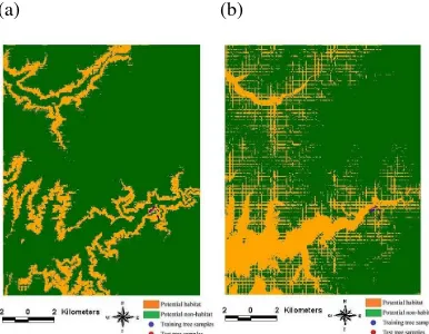
values of four models lifted back to almost the same values as those in SS-1 from SS-2 or even better, and the four models still kept the same order in accuracy as that in SS-1. As the first data-merged models built in SS-3 were applied to a larger area in SS-4 including Tong-Mao Mountain, with 10 km away from the three sites at Huisun, the kappa values of MAXENT and DA declined to near zero, as well as GARP and GLM could not work possibly due to a limit on the size of data layer, a big difference in the domain values of predictor variables between Huisun and Tong Mao, or some other possible unknown factors which we will figure out later. In contrast, the kappa value of MAXENT in SS-5 rebounded strikingly as the second data-merged models built in SS-5 were applied to the same area as that in SS-4 (Table 2), while that of DA rose back slightly. Consequently, it was unlikely to accurately extend spatial patterns of CFs from the Huisun area to Tong-Mao Mountain area with 10 km gap or to the entire study area encompassing Huisun by predictive models merely based on topographic (indirectly operating) variables.
The models, either base models in SS-1 or the first data-merged models in SS-3, accurately predicted the potential habitats of CFs in Huisun, and substantially reduced the area of field survey to less than 10% of the entire study area, even less than 2.5% with MAXENT (Tables 3 and 4 and Figure 2). In Huisun study area, all the potential CF habitats predicted occurred in the Kuan-Dau watershed, and none occurred in the Tong-Feng watershed because of remarkable differences in humidity and solar illumination between them. The outcome had been proved true by field surveys through which almost no cycad-ferns were found in the Tong-Feng watershed. In contrast, neither the first data-merged models in SS-3 nor the second data-merged models in SS-5 could not accurately extrapolated CF spatial patterns when they were applied to the larger area encompassing Ton Mao Mountain. Consequently, they could not reduce the area of field survey to less than 10% of the entire study area, even greater than 25% with DA (Tables 5 and 6 and Figure 3).
MAXENT GARP GLM DA
Class
SS1 SS2 SS3 SS1 SS2 SS3 SS1 SS2 SS3 SS1 SS2 SS3 Overall (%) 97 97 96 88 88 95 95 95 95 86 86 87 Training
Kappa .89 .89 .88 .62 .62 .87 .83 .83 .85 .63 .63 .68
Overall (%) 95 90 95 88 78 91 96 92 92 85 84 85 Test
Kappa .84 .46 .86 .60 .12 .77 .70 .70 .77 .66 .55 .62
Table 1 SS-1, SS-2, SS-3: the accuracies of the models with elevation, slope, and terrain position variables for predicting the potential habitat of CFs.
MAXENT GARP GLM DA
Class
SS4 SS5 SS4 SS5 SS4 SS5 SS4 SS5
Overall (%) 86 91 — — — — 70 69
Training
Kappa .64 .75 — — — — .34 .33
Overall (%) 82 91 — — — — 64 66
Test
Kappa .06 .75 — — — — .05 0.25
MAXENT GARP GLM DA Class
Area (ha) % Area (ha) % Area (ha) % Area (ha) %
Habitat 290 1.7 1406 8.2 991 5.8 1582 9.2
Non-Habitat 16846 98.3 15730 91.8 16145 94.2 15554 90.8
Sum 17136 100 17136 100 17136 100 17136 100
Table 3 SS-1: distribution statistics of predictive maps of the CF potential habitat generated from the models with elevation, slope, and terrain position variables.
MAXENT GARP GLM DA
Class
Area (ha) % Area (ha) % Area (ha) % Area (ha) %
Habitat 374 2.2 998 5.8 1006 5.9 1527 8.9
Non-Habitat 16762 97.8 16138 94.2 16130 94.1 15609 91.1
Sum 17136 100 17136 100 17136 100 17136 100
Table 4 SS-3: distribution statistics of predictive maps of the CF potential habitat generated from the first data-merged models with elevation, slope, and terrain position variables.
MAXENT DA
Class
Area (ha) % Area (ha) %
Habitat 4395 15.4 7549 26.46
Non-Habitat 24130 84.6 20976 73.54
Sum 28525 100 28525 100
Table 5 SS-4: distribution statistics of predictive maps of the CF potential habitat generated from the two models with elevation, slope, and aspect variables.
MAXENT DA
Class
Area (ha) % Area (ha) %
Habitat 2924 10.3 7567 26.53
Non-Habitat 25601 89.7 20958 73.47
Sum 28525 100 28525 100
Table 6 SS-5: distribution statistics of predictive maps of the CF potential habitat generated from the second data-merged models with elevation, slope, and aspect variables.
(a) (b) (c) (d)
Figure 2 SS-3: four models for mapping the potential habitat of cycad-ferns in the Huisun study area, (a) MAXENT; (b) GARP; (c) GLM; (d) DA.
(a) (b)
5. CONCLUSIONS
The study developed the four models that related the known CF sites to habitat characteristics and predicted the plant’s potential sites in the study area. For the case of Huisun area, the four models accurately predicted the potential habitats of CFs in Huisun, and substantially reduced the area of field survey to less than 10% of the Huisun study area, and were implemented efficiently. As a result, they were well suited for spatial distribution modeling of CFs. MAXENT was the best because it had highest accuracy and reliability among them. More importantly, they can prioritize either the field-survey areas where it is viable to collect fine spatial-resolution microclimatic, edaphic, or biotic data for refining predictions of potential habitat in the later rounds of SDM or search areas for new population discovery under the conditions of limited funding and manpower. However, the outcome showed that it is unlikely to accurately extrapolate the spatial patterns of CFs from one area to another area with a big separation or to a larger area encompassing the original one by predictive models merely based on topographic variables, as in the case of our entire study area. Follow-up studies will attempt to incorporate proxy indicators that can be extracted from hyperspectral images or LIDAR DEM and substitute for direct parameters, and so that predictive models are applicable on a broader scale.
6. REFERENCES
Asner, G. P., M. O. Jones, R. E. Martin, D. E. Knapp, R. F. Hughes, 2008, Remote sensing of native and invasive species in Hawaiian forests. Remote Sensing of Environment, 112, pp. 1912–1926.
Barve, N., V. Barve, A. Jimenez-Valverde, A. Lira-Noriega, S. P. Maher, A. T. Peterson, J. Soberon and F. Villalobos, 2011, The crucial role of the accessible area in ecological niche modeling and species distribution modeling. Ecological Modelling, 222, pp. 1810–1819.
Cayuela L., D. J. Golicher, A. C. Newton, M. Kolb, F. S. de Alburquerque, E. J. M. M. Arets, J. R. M. Alkemade and A. M. Pérez, 2009. Species distribution modeling in the tropics: problems, potentialities, and the role of biological data for effective species conservation. Tropical
Conservation Science, 2 (3), pp. 319–352
Côté, I. M. and J. D. Reynolds, 2002. Predictive ecology to the rescue? Science, 298 (5596), pp. 1181–1182. Manion, C. Moritz, M. Nakamura, Y. Nakazawa, J. McC. Overton, A. T. Peterson, S. J. Phillips, K. S. Richardson, R. Scachetti-Pereira, R. E. Schapire, J. Sobero´n, S. Williams, M. S. Wisz and N. E. Zimmermann, 2006. Novel methods improve prediction of species’ distributions from occurrence data. Ecography, 29, pp. 129–151.
Guisan A., C. H. Graham, J. Elith, F. Huettmann and the NCEAS Species Distribution Modelling Group, 2007. Sensitivity of predictive species distribution models to
change in grain size. Diversity and Distributions, 13, pp.
332–340.
Guisan, A., T. C. Edwards Jr and T. Hastie, 2002. Generalized linear and generalized additive models in studies of
species distributions: setting the scene. Ecological Modelling 157, pp. 89–100.
Guisan, A. and N. E. Zimmermann, 2000. Predictive habitat distribution models in ecology. Ecological Modelling, 135, pp. 147–186.
Guisan, A. and W. Thuiller, 2005. Predicting species distribution: offering more than simple habitat models. Ecology Letters, 8, pp. 993–1009.
Hernandez P. A., C. H. Graham, L. L. Master and D. L. Albert, 2006. The effect of sample size and species characteristics on performance of different species distribution modeling methods. ECOGRAPHY, 29, pp. 773–785.
Ke, Y., L. J. Qackenbush, J. Im., 2010. Synergistic use of QuickBird multispectral imagery and LIDAR data for object-based forest species classification. Remote Sensing of Environment, (114), pp. 1141–1154.
Lillesand, T. M., R. W. Kiefer and J. W. Chipman, 2008. Remote Sensing and Image Interpreatation, 6th ed, John Wiley & Sons, Inc., pp.591.
Lowell, K., 1991. Utilizing discriminant function analysis with a geographical information system to model ecological succession spatially. International Journal of Geographical Information System, 5 (2), pp. 175–191.
Lu, J. C., Y. J. Liu and M. Y. Chen, 1986. Brainea insignis a new distribution and plant community composition in Taiwan. Quarterly of journal Chinese Forestry, 19 (1), pp. 121–126.
Pearson, R. G., C. J. Raxworthy, M. Nakamura and A. T. Peterson, 2007. Predicting species distributions from small numbers of occurrence records: a test case using cryptic geckos in Madagascar. J. Biogeo 34, pp.102–117. Pereira, J. M. C. and R. M. Itami, 1991. GIS-based habitat
modeling using logistic multiple regression: a study of the Mt. Graham red squirrel. Photogrammetric Engineering & Remote Sensing, 57 (11), pp. 1475–1486.
Phillips, S. J., R. P. Anderson and R. E. Schapire, 2006. Maximum entropy modeling of species geographic distributions, Ecol. Model, 190, pp. 231–259 Photogrammetric Engineering & Remote Sensing, 62 (11), pp. 1269–1279.
Stockwell, D. R. B. and I. R. Noble, 1992. Induction of sets of rules from animal distribution data: a robust and informative method of data analysis, Math. Comput. Simul, 33, pp. 385–390.
Stockwell, D. and D. Peters, 1999. The GARP modelling system: problems and solutions to automated spatial prediction. International Journal of Geographical Information Science 13, pp. 143–158.
Su, H. J., 1987. Forest habitat factors and their quantitative assessment. Quarterly Journal of Chinese Forestry, 20, 1–28. (In Chinese with English abstract)