*Corresponding author. Tel.:#886-35-712121ext.57125. E-mail address:[email protected] (C. Chiang).
Order splitting under periodic review inventory systems
Chi Chiang*
Department of Management Science, National Chiao Tung University, Hsinchu, Taiwan, Republic of China Accepted 12 April 2000
Abstract
Most research on order splitting have focused on the reduction of safety stock in the multiple sourcing setting. Moreover, all works study the use of order splitting for the continuous review inventory systems. In this paper, we investigate the possibility of the multiple-delivery arrangement in the sole sourcing environment. In addition, we concentrate on the reduction of cycle stock for periodic review systems. We show that splitting an order into multiple deliveries can signi"cantly reduce the total cost especially if the cost of despatching an order for an item is not small. Although the use of information technology such as EDI decreases the ordering cost and thus shortens the period length, order splitting remains a cost-e!ective approach as long as the cost of despatching an order is not close to zero. ( 2001 Elsevier Science B.V. All rights reserved.
Keywords: Inventory; Order-splitting; JIT; Periodic review; Information technology
1. Introduction
The use of order splitting during an order cycle seems to have received much attention recently. For example, Kelle and Silver [1] analyze the safety stock reduction by order splitting assuming the Weibull-distributed lead times, and Sculli and
Shum [2] present numerical results on the e!ect of
order splitting on the lead-time demand. Ramasesh et al. [3], Lau and Zhao [4], and Chiang and Benton [5] further develop a total cost model, respectively to obtain the optimal reorder point and order quantity jointly. However, these works have focused on the reduction of safety stock in the multiple sourcing setting. In comparision with cycle stock, safety stock is only a small portion of
a company's inventory. In a recent paper, Chiang
and Chiang [6] propose the arrangement of multiple deliveries during each order cycle, and consider the reduction of cycle stock in the sole sourcing environment. All of these studies have concentrated on the use of order splitting for con-tinuous review inventory systems. In this paper, we investigate the use of order splitting during each period (also called order cycle thereafter) for
peri-odic review (R,S) systems (without a reorder point).
In addition, we focus on the reduction of cycle stock in the sole sourcing setting. Our research also provides a rationale for the just-in-time (JIT) frequent-delivery approach.
In a typical periodic review system, an order
quantity which brings the inventory level to S is
placed with a speci"c vendor whenever inventory is
reviewed every period of lengthR. Such an
operat-ing policy, known as a replenishment cycle system, is often found in practice (see, e.g. [7]). Although the use of computer systems nowadays has made
continuous review systems more popular, periodic review systems are still applied in many situations (see, e.g. [8]). Often, periodic systems are found to have the review periods which are longer than the supply lead times. For instance, a retailer may place regular replenishment orders biweekly while the supply lead time is of the order of one week.
It is generally assumed in a periodic system that the whole order quantity from the supplier arrives in a single delivery in each period. It is possible, however, that the buyer could have the supplier agree to order splitting so that portions of an order
quantity arrive at the receiving point at di!erent
times of a period. For companies who work with their suppliers on a long-term relationship, this multiple-delivery approach is particularly feasible and useful. For example, Hotai Motor Co. Ltd., the distributor of Toyota products (and the largest auto distributor) in Taiwan, has recently adopted this multiple-delivery approach, which will be com-monly used in the future by other auto distributors. Hotai Motor Co. Ltd. orders thousands of service parts for domestically manufactured cars (such as Toyota Corona Exsior and Tercel) monthly from six major suppliers (not including the Toyota Mo-tor Company in Japan) (manufacturing of these
cars is in a di!erent company). Each of the six
suppliers makes at least 10 deliveries (low-usage items are shipped less frequently than high-usage items) per month to the central warehouse of Hotai Motor Co. Ltd.
Apparently, the bene"t of this multiple-delivery
approach is the reduction in the average cycle stock, while the disadvantage of this approach is that ordering costs (which include transportation and inspection costs) may increase. The major goal of this research is to develop a multiple-delivery
model and evaluate this tradeo!. In addition, if it
bene"ts the buyer to arrange multiple deliveries with the supplier, does there exist an optimal num-ber of deliveries per order cycle? This research also investigates this issue.
We assume that bothRandSare decision
vari-ables. In addition, we assume that lead time is constant, demand is non-negative and indepen-dently distributed in disjoint time intervals, and
that demand during a time interval of length qis
normally distributed with mean kq and variance
p2q. Note that in practiceRis often predetermined
by the"rm. For example, a retailer may coordinate
a group of items to a distribution center weekly or biweekly. Also, vendors in a department store often make routine visits to customers to take fresh orders [8]. There may exist other practical or or-ganizational considerations (see, e.g. [9]). In this
paper, however, we assume that R is a variable
inside the model.
In addition, as the supply chain management of
materials has been a trend in industry, some"rms
have invested in information technology to reduce the communication and transaction time among trading partners. The use of electronic data inter-change (EDI) in inventory control systems has been
particularly noteworthy and the bene"ts of reduced
logistics and order processing costs are reported [10]. In this paper, we also discuss the impact of the reduction of ordering costs on the shortening of the review periods and on the performance of the
multiple-delivery model, after the"rm and its
sup-plier(s) have decided to invest in EDI (i.e., the deci-sion of establishing an EDI-based inventory system has been made and is not considered inside the model).
This paper is organized as follows. First, we
brie#y review the ordinary single-delivery
approach under periodic review systems. Then we present a two-delivery model, which is followed by some computational results. Next, we generalize the analysis to the multiple-delivery model. Finally, this paper ends with the conclusion.
2. Review of the single-delivery approach
We "rst review the ordinary single-delivery
approach. Let ¸
1 be the constant lead time and
h
1(>1) the probability density function (PDF) for
the demand >
1 over a period of length R. Then
h
1(>1) is N(kR,p2R). Suppose that we review
inventory at the time pointtand>
1is the demand
during the preceding period (t!R,t). Then we will
order >
1 and raise the inventory position up to
S which should be large enough to meet the
de-mand for the upcoming time interval of length
R#¸
1. LetB(¸1) be the average backorder that
Fig. 1. A two-delivery model.
andG()) is the partial expectation function tabled
in Brown [11] or Silver and Peterson [7]. Instead of having to estimate the backorder cost, we use a service level (SL) constraint for the objective
func-tion (as in [6]). Service level is de"ned as the
per-centage of demand to be served directly from stock. For the single-delivery approach, service level is given by
SL"100!100B(¸1)
kR . (3)
LetDbe the average annual demand,Athe"xed
ordering cost,Jthe review cost, andhthe annual
carrying cost per unit. To simplify the notation, we incorporate the review cost into the ordering cost,
i.e., A also includes the review cost. The ordering
costA, as described by Lau and Zhao [4], consists
of two components. One is the cost of despatching an order for an inventory item each time, denoted
byO, such as administrative and processing costs
(note that the review cost is included in O). The
other is the cost of receiving an incoming
procure-ment, denoted byI, such as costs of transportation,
handling and inspection of the procurement after it
arrives, etc. O and I togeter constitute the "xed
ordering cost A (i.e., A"O#I). The use of
in-formation technology such as EDI will decrease
Oand thus shorten the period lengthR. In Section
4, we will investigate this issue. As the average
amount ordered per period is kR and the safety
stock is S!k¸
1!kR, the decision problem for
the single-delivery model can be expressed by
MinC(R,S)"[D(O#I)/kR]
wheretis a preassigned service level. Note that the
expression for average on-hand inventory is only an approximation, i.e., it assumes that the average backorder level is quite small (see, e.g. [12]). Given the nature of the problem, the optimal solution will automatically satisfy constraint (5) at equality. To
"nd the optimal R and S, we use (5) to "nd the
optimalSfor a given value ofR. Then we tabulate
the total cost as a function ofR to determine the
optimalR[12].
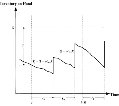
3. A two-delivery model
We now present a two-delivery model for the
periodic review (R,S) system. Let ¸
2 (which is
smaller than R) be the inter-arrival time between
the"rst and second shipments. We suppose that we
order>
1(i.e., demand during the preceding period)
at the review epoch t and the supplier agrees to
deliver part of the order quantity after time¸
1and
the remaining part after time¸
1#¸2(see Fig. 1).
(Notice that¸
1#¸2 need not be less than R as
shown in Fig. 1.) Let (1!w)kRbe the size of the
second shipment and thus >
1!(1!w)kR is the
size of the"rst shipment (note that the average size
of the"rst shipment iswkR). The idea is to raise the
inventory up to S!(1!w)kR in the "rst
ship-ment. It is assumed that >
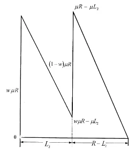
Fig. 2. Average cycle stock of the two-delivery model.
>
1should be less than (1!w)kR, there is only one
shipment of size>
1delivered after¸1#¸2.>1is
at least (1!w)kRif¸
2 is not too short so thatw
is very small (the fact that w depends on ¸
2
is shown in the following computation). Intuitively, to make the two-delivery arrangement attractive,
the inter-arrival time ¸
2 should not be too
short, since otherwise the reduction in the average cycle stock (to be explained below) would be very small and the two-delivery approach may only re-sult in an increase in the material handling cost (part of the ordering cost). It is assumed for the time
being that ¸
2 is "xed. Later we will explore how
¸
2 can have an impact upon the total cost of the
buyer.
single-delivery approach, it is generally assumed
that the order placed at the review epochtwould
clear all the shortages (if any) at the time of arrival (see, e.g. [12]). In the two-delivery model, shortages
may not be all cleared at timet#¸
1(since part of
the order arrives at time t#¸
1#¸2). More
im-portantly, shortages can occur between timet#¸
1
and t#¸
1#¸2. Thus, we need to compute the
shortages that might build up before the receipt of the second shipment. Note that there is the possibil-ity of double-counting the same shortages as long as a shipment could not clear all the shortages at the time of arrival. Although this should rarely happen (since the average backorder level is quite small), we assume that we are willing to accept
possible double-counting [6]. LetB(¸
2) denote the
average backorder that might build up before the recipt of the second shipment. For the two-delivery approach, the service level is given by
SL"100!100B(¸1)#B(¸2)
Also, if we let the arrival of the"rst shipment of
an order initiate a cycle, then a cycle consists of two
time intervals of length¸
2andR!¸2(see Fig. 1).
The average cycle stock is wkR!k¸
2/2 for the
time interval of length ¸
2 and kR/2!k¸2/2
for the time interval of lengthR!¸
2 (see Fig. 2).
Thus, the overall average cycle stock is
kR/2!(1!w)k¸
2. By splitting an order into two
deliveries, we see that the average cycle stock is
reduced by (1!w)k¸
2(ifRremains the same as in
the single-delivery model).
On the other hand, when two deliveries of an order are arrenged with the supplier, the ordering cost may increase. While the cost of despatching an order is unchanged, the cost of receiving incoming procurements may nearly double. We assume that when two deliveries of an order are arranged with
the supplier, the ordering cost becomesO#2I.
It follows that the decision problem for the two-delivery model discussed above is expressed by
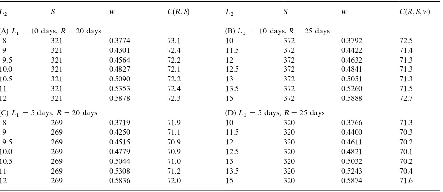
Table 1
E!ect of the inter-arrival time¸
2on the performance of the two-delivery model. Data:k"10 units/day,p"2 units, 1 year"250 days, A"$2(O"I"$1),t"99.90,h"$0.5/unit/year
¸
2 S w C(R,S) ¸2 S w C(R,S,w)
(A)¸
1"10 days,R"20 days (B)¸1"10 days,R"25 days
8 321 0.3774 73.1 10 372 0.3792 72.5
9 321 0.4301 72.4 11.5 372 0.4422 71.4
9.5 321 0.4564 72.2 12 372 0.4632 71.3
10.0 321 0.4827 72.1 12.5 372 0.4841 71.3
10.5 321 0.5090 72.2 13 372 0.5051 71.3
11 321 0.5353 72.4 13.5 372 0.5260 71.5
12 321 0.5878 72.3 15 372 0.5888 72.7
(C)¸
1"5 days,R"20 days (D)¸1"5 days,R"25 days
8 269 0.3719 71.9 10 320 0.3766 71.3
9 269 0.4250 71.1 11.5 320 0.4400 70.3
9.5 269 0.4515 70.9 12 320 0.4611 70.2
10.0 269 0.4779 70.9 12.5 320 0.4821 70.1
10.5 269 0.5044 71.0 13 320 0.5032 70.2
11 269 0.5308 71.2 13.5 320 0.5243 70.4
12 269 0.5836 72.0 15 320 0.5874 71.6
s.t.
Note that (10) can be easily shown to be convex
with respect toS andw(for a givenR). Given the
nature of the problem, the optimal solution will always have constraint (10) held at equality. By formulating the Lagrangian
and setting the derivatives with respect toS,wand
jequal to zero, we can obtain
¸
cumulative distribution function for the standard normal variable. It is evident from (12) and (13) that
the optimal S and w (given a certain R) do not
depend on the values ofO, I, and h. To "nd the
optimal combination ofR,S, andw, we use (12) and
(13) to"nd the optimalSandwfor a givenR. Then
we tabulate the total cost as a function of R to
determine the optimalR.
4. Computational results
We investigate the e!ect of the inter-arrival time
¸
2on the performance of the two-delivery model.
We also examine the e!ect of cost parameters,
demand variability, and service level on the perfor-mance of the two-delivery model relative to the single-delivery model.
4.1. Ewect of the inter-arrival time
We"rst investigate the e!ect of¸
2on the
perfor-mance of the two-delivery model. It appears from Table 1 that the total cost is at a minimum when ¸
2 is approximately equal to R/2. Note that this
result is also obtained under other levels of¸
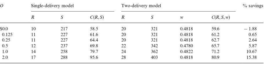
Table 2
Single-delivery model versus two-delivery model under di!erent levels ofO. Data:k"10 units/day,p"2 units, 1 year"250 days, ¸
1"10 days,¸2"R/2,I"$1,h"$0.5/unit/year,t"99.90
O Single-delivery model Two-delivery model % savings
R S C(R,S) R S w C(R,S,w)
$0.0 10 217 58.5 20 321 0.4818 59.6 !1.88
0.125 11 227 61.6 20 321 0.4818 61.2 0.65
0.25 11 227 64.4 20 321 0.4818 62.7 2.64
0.5 12 237 69.8 22 342 0.4780 65.7 5.87
1.0 14 258 79.7 24 362 0.4822 71.2 10.67
2.0 17 288 95.6 28 403 0.4818 80.9 15.38
Table 3
Single-delivery model versus two-delivery model under di!erent levels ofI. Data:k"10 units/day,p"2 units, 1 year"250 days, ¸
1"10 days,¸2"R/2,O"$1,h"$0.5/unit/year,t"99.90
I Single-delivery model Two-delivery model % savings
R S C(R,S) R S w C(R,S,w)
$0.25 11 227 64.4 17 291 0.4744 52.7 18.17
0.5 12 237 69.8 20 321 0.4818 59.6 14.61
1.0 14 258 79.7 24 362 0.4822 71.2 10.67
2.0 17 288 95.6 31 433 0.4862 89.5 6.38
4.0 22 339 121.3 41 535 0.4861 117.2 3.38
8.0 30 420 160.0 51 697 0.4895 157.8 1.37
R, although the computations are not shown here.
We are unable to prove this result due to the partial expectation functions involved. However, we could explain as follows. As mentioned above, we can let
the arrival of the"rst shipment of an order initiate
a cycle. Then if ¸
2"R/2, the arrival of second
shipment is exactly halfway through a cycle. It is as though we place an order (in a single shipment)
every period of lengthR/2 and the arrival epochs
would be the same. For computational purposes, it
is much easier to"x¸
2atR/2 and"nd the optimal
combination of R,S and w, instead of treating
¸
2also as a variable. Moreover, it is easy for both
the buyer and the supplier to implement the
two-delivery contract when¸
2 is simply "xed atR/2.
Consequently, we set ¸
2"R/2 in the
computa-tions thereafter.
4.2. Ewect of cost parameters
We next consider the e!ect of cost parameters.
Note that the cost structure is characterized by the
ratio ofA/hor (O#I)/h. Thus, we"x the value of
hto investigate the e!ect of the amount ofA(relative
toh) on the performance of the two-delivery model.
Since A"O#I, we vary the value of O and I,
respectively, to examine their e!ect. As we see from
Tables 2 and 3, the two-delivery model becomes
more attractive asO increases andIdecreases,
re-spectively (other things being equal). These results came with no surprise. Since the ordering cost equals
O#2Iin the two-delivery model, a smallerIresults
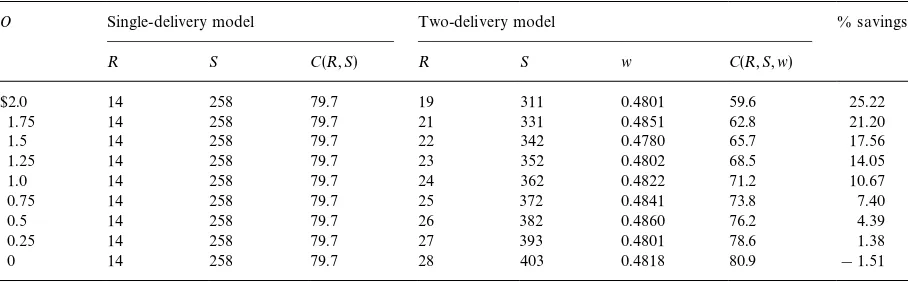
Table 4
Single-delivery model versus two-delivery model under di!erent levels of the ratioO/(O#I). Data:k"10 units/day,p"2 units, 1 year"250 days,¸
1"10 days,¸2"R/2,A"O#I"$2,h"$0.5/unit/year,t"99.90
O Single-delivery model Two-delivery model % savings
R S C(R,S) R S w C(R,S,w)
$2.0 14 258 79.7 19 311 0.4801 59.6 25.22
1.75 14 258 79.7 21 331 0.4851 62.8 21.20
1.5 14 258 79.7 22 342 0.4780 65.7 17.56
1.25 14 258 79.7 23 352 0.4802 68.5 14.05
1.0 14 258 79.7 24 362 0.4822 71.2 10.67
0.75 14 258 79.7 25 372 0.4841 73.8 7.40
0.5 14 258 79.7 26 382 0.4860 76.2 4.39
0.25 14 258 79.7 27 393 0.4801 78.6 1.38
0 14 258 79.7 28 403 0.4818 80.9 !1.51
On the contrary, a smallerOsaves the
two-deliv-ery model vtwo-deliv-ery little of the ordering cost and thus
makes it less e!ective. This has a very important
implication. As we mentioned before, the use of
EDI in inventory systems will lowerOand thus the
optimal period lengthRis shortened, as can be seen
from Table 2. If we assume that the "rm and its
supplier(s) have made an investment in EDI, the use of order splitting does not appear particularly
at-tractive as Ois decreased to a smaller level in the
long run. Nevertheless, the"rm bene"ts from the
use of the delivery approach, since the two-delivery approach obtains a lower total cost than the traditional single-delivery approach as long as
Ois not decreased to a level of near zero. This result
also is apparent from Table 4. If we"x the value of
Abut change the proportion ofOinA, we see that
the two-delivery approach yields a smaller
percent-age cost savings as the ratio of O/Adecreases to
zero. In an extreme case of O/A+0, splitting an
order into two deliveries during each cycle will increase the total cost.
As a note, the two-delivery approach yields a
larger R than the single-delivery model, although
the inter-arrival time¸
2between the two deliveries
is shorter than the optimalRof the single-delivery
model. This implies that the buyer will order a larger quantity and thus is more likely to ob-tain quantity discounts under the two-delivery model.
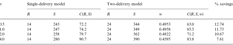
4.3. Ewect of demandvariability and service level
Next, we examine the e!ect of demand variability
and service level on the performance of the single-delivery model versus the two-single-delivery model. It appears from Tables 5 and 6 that the two-delivery
model performs better under lower levels of p or
t(other things being equal). This is because there
are two stockout possibilities (one more than the single-delivery model) during each order cycle in the two-delivery model. Thus, the two-delivery model is less vulnerable to stockouts if demand variability or service level is low. This agrees with the"nding of Chiang and Chiang [6].
5. A multiple-delivery model
We consider the possibility of the arrengement of
n shipments during each order cycle. Let
¸
i"R/n, i"2,2,n, be the inter-arrival time
be-tween the (i!1)th andith shipments. We suppose
that the supplier agrees to deliver theith shipment
after +ij/1¸
j, i"1,2,n, and the "rst shipment
has size>
1!(1!w1)kR(note again that the
aver-age size of the"rst shipment isw
1kR), the second
shipment has sizew
2kR,2, the (n!1)th shipment
has size w
n~1kR, and the nth shipment has size
(1!+n~1j/1w
j)kR. LetB(¸i),i"2,2,nbe the
Table 5
Single-delivery model vs. two-delivery model under di!erent levels ofp. Data:k"10 units/day, 1 year"250 days,¸
1"10 days, ¸
2"R/2,A"$2, (O"I"$1),t"99.90,h"$0.5/unit/year
p Single-delivery model Two-delivery model % savings
R S C(R,S) R S w C(R,S,w)
0.5 14 243 72.2 24 344 0.4953 63.0 12.74
1.0 14 247 74.2 24 349 0.4958 65.5 11.73
2.0 14 258 79.7 24 362 0.4822 71.2 10.67
4.0 14 280 90.7 24 390 0.4595 83.8 7.61
Table 6
Single-delivery model vs. two-delivery model under di!erent levels oft. Data:k"10 units/day,p"2 units, 1 year"250 days,¸ 1"10
days,¸
2"R/2,A"$2(O"I"$1),h"$0.5/unit/year
t Single-delivery model Two-delivery model % savings
R S C(R,S) R S w C(R,S,w)
95.00 14 235 68.2 24 336 0.5066 59.6 12.60
99.00 14 247 74.2 24 350 0.4895 65.6 11.59
99.90 14 258 79.7 24 362 0.4822 71.2 10.67
99.99 14 266 83.7 24 371 0.4765 75.3 10.03
receipt of theith shipment. Then,
B(¸
We assume that the ordering cost isO#nIwhen
nshipments during each cycle are arrenged with the
supplier. Noticing that the average cycle stock is
reduced by (1!w
To "nd the optimal combination of S and w j, j"1,2,n!1, for a given R, we formulate the Lagrangian of this multiple-delivery model and set
the derivatives with respect toSandw
Table 7
Two-delivery model versus three-delivery model under di!erent levels of the ratioO/(O#I). Data:k"10 units/day,p"2 units, 1 year"250 days,¸
1"10 days,O#I"$2,h"$0.5/unit year,t"99.90
O Two-delivery model Three-delivery model % savings
R S w C(R,S,w) R S w
1 w2 C(R,S,w1,w2)
$2.0 19 311 0.4801 59.6 24 364 0.3050 0.3463 51.1 14.26
1.5 22 342 0.4780 65.7 29 415 0.3076 0.3458 60.6 7.76
1.0 24 362 0.4822 71.2 33 456 0.3086 0.3446 68.7 3.51
0.5 26 382 0.4860 76.2 37 496 0.3120 0.3462 75.8 0.52
0 28 403 0.4818 80.9 41 537 0.3124 0.3448 82.2 !1.61
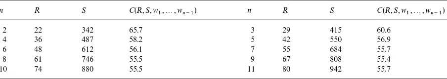
Table 8
Multiple-delivery models. Data:k"10 units/day,p"2 units, 1 year"250 days,¸
1"10 days,O"$1.5,I"$0.5,h"$0.5/unit/year,
t"99.90
n R S C(R,S,w
1,2,wn~1) n R S C(R,S,w1,2,wn~1)
2 22 342 65.7 3 29 415 60.6
4 36 487 58.2 5 42 550 56.9
6 48 612 56.1 7 55 684 55.7
8 61 746 55.5 9 67 808 55.4
10 74 880 55.5 11 80 942 55.7
(see the appendix for details). Since ¸
i"R/n, i"2,2,n, it follows from (20) thatk1"k2"2 "k
n. Hence, we can use the following procedure to
obtain the optimalS andw
j,j"1,2,n!1.
Step 1. Substitutek
2"k1,2,kn"k1 into (21)
to obtaink
1 and thusS.
Step 2. Usek
i"k1,i"2,2,n, to obtainwj by
using (15),j"1,2,n!1, respectively.
We then tabulate the total cost as a function of
Rto determine the bestR. Table 7 gives the
com-putational results for the relative performance of the two-delivery model versus the three-delivery model. As we see, the total cost may be further reduced if we split an order into three deliveries during each cycle.
A question arises at this point: does there exist an
optimal numberof deliveries per cycle that results in minimum total cost (as in [6]). To investigate this, we carry out the computation further. As we see, for example, the optimal number of deliveries per cycle is 9 in Table 8. This also illustrates the frequent-delivery approach that Hotai Motor Co. Ltd. (as mentioned in the introduction) employs to reduce the inventory carrying cost. As Hotai Motor Co.
Ltd. works with its major suppliers on a long-term relationship, the ordering cost of an item is small. Often, delivery of a split procurement for an item is part of a joint shipment which includes hundreds of items, and there is no inspection after the procure-ment arrives. The suppliers also absorb some of the transportation cost.
In summary, if the ordering cost structure agrees with what we assume, the buyer should consider negotiating an optimal number of deliveries for each cycle with the supplier.
6. Conclusion
the period length, order splitting remains a
cost-e!ective approach as long as the cost of
despatch-ing an order is not close to zero. Moreover, we show that there exists an optimal number of delive-ries per cycle such that the lowest total cost is obtained. As very few assumptions are made in this
research, "rms can apply the approach of order
splitting in practice immediately, as long as mul-tiple shipments of an order can be arranged with suppliers. Finally, we should note that this research also provides a rationale for the JIT frequent-deliv-ery approach.
Appendix A
In this appendix, we derive expression (20) of Section 5. The Lagrangian including (16) and (17)
with a multiplierjis
[D(O#nI)/kR]#h
G
S!k¸Di!erentiating it with respect toSand setting the
derivative equal to zero, we obtain
j"h/(P(k
1)#P(k2)#2#P(kn)). (A.1)
Next, we di!erentiate the Lagrangian with respect
tow
n~1, set it to zero, and substitute (A.1) into the
expression to give
¸
n/R"P(kn)/(P(k1)#P(k2)#2#P(kn)). (A.2)
Then, we di!erentiate the Lagrangian with respect
w
n~2, set it to zero, and substitute (A.1) into the
expression to give
(¸
n~1#¸n)/R"(P(kn~1)#P(kn))/(P(k1)
#P(k
2)#2#P(kn)),
and substitute (A.2) into the above expression to yield
¸
n~1/R"P(kn~1)/(P(k1)#P(k2)#2#P(kn)).
(A.3)
Continue this way and di!erentiate with respect to
w
n~3,2, and w1 to obtain respectively
¸
n~2/R"P(kn~2)/(P(k1)#P(k2)#2#P(kn)), F
¸
2/R"P(k2)/(P(k1)#P(k2)#2#P(kn)),
The above expressions together with (A.2) and (A.3) are expression (20) in Section 5.
References
[1] P. Kelle, E.A. Silver, Safety stock reduction by order split-ting, Naval Research Logistics 37 (1990) 725}743. [2] D. Sculli, Y. Shum, Analysis of a continuous review stock
control model with multiple suppliers, Journal of Opera-tional Research Society 41 (1990) 873}877.
[3] R.V. Ramasesh, J.K. Ord, J.C. Hayya, A.C. Pan, Sole versus dual sourcing in stochastic lead-time (s, Q) inven-tory models, Management Science 37 (1991) 428}443. [4] H. Lau, L. Zhao, Optimal ordering policies with two
suppliers when lead times and demands are all stochastic, European Journal of Operational Research 68 (1993) 120}133.
[5] C. Chiang, W.C. Benton, Sole sourcing versus dual sourc-ing under stochastic demands and lead times, Naval Research Logistics 41 (1994) 609}624.
[6] C. Chiang, W.C. Chiang, Reducing inventory costs by order splitting in the sole souring environment, Journal of the Operational Research Society 47 (1996) 446}456. [7] E.A. Silver, R. Peterson, Decision Systems for Inventory
Management and Production Planning, Wiley, New York, 1985.
[8] R.B. Chase, N.J. Aquilano, Production and Operations Management, Irwin, Homewood, IL, 1997.
[9] M.K. Starr, Operations Management, Boyd & Fraser, MA, 1996.
[10] T. Lester, Squeezing the supply chain, Management Today (1992) 68}70.
[11] R.G. Brown, Decision Rules for Inventory Management, Holt, Rinehart, and Winston, New York, 1967.