Modular Symmetry and Fractional Charges
in
N
= 2 Supersymmetric Yang–Mills
and the Quantum Hall Ef fect
⋆Brian P. DOLAN †1†2 †1
Department of Mathematical Physics, National University of Ireland, Maynooth, Ireland
†2
School of Theoretical Physics, Dublin Institute for Advanced Studies, 10, Burlington Rd., Dublin, Ireland
E-mail: [email protected]
URL: http://www.thphys.nuim.ie/staff/bdolan/
Received September 29, 2006, in final form December 22, 2006; Published online January 10, 2007 Original article is available athttp://www.emis.de/journals/SIGMA/2007/010/
Abstract. The parallel rˆoles of modular symmetry inN = 2 supersymmetric Yang–Mills and in the quantum Hall effect are reviewed. In supersymmetric Yang–Mills theories mod-ular symmetry emerges as a version of Dirac’s electric – magnetic duality. It has significant consequences for the vacuum structure of these theories, leading to a fractal vacuum which has an infinite hierarchy of related phases. In the case ofN = 2 supersymmetric Yang–Mills in 3 + 1 dimensions, scaling functions can be defined which are modular forms of a subgroup of the full modular group and which interpolate between vacua. Infra-red fixed points at strong coupling correspond to θ-vacua with θ a rational number that, in the case of pure SUSY Yang–Mills, has odd denominator. There is a mass gap for electrically charged par-ticles which can carry fractional electric charge. A similar structure applies to the 2 + 1 dimensional quantum Hall effect where the hierarchy of Hall plateaux can be understood in terms of an action of the modular group and the stability of Hall plateaux is due to the fact that odd denominator Hall conductivities are attractive infra-red fixed points. There is a mass gap for electrically charged excitations which, in the case of the fractional quantum Hall effect, carry fractional electric charge.
Key words: duality; modular symmetry; supersymmetry; quantum Hall effect
2000 Mathematics Subject Classification: 11F11; 81R05; 81T60; 81V70
1
Introduction
The rˆole of the modular group as a duality symmetry in physics has gained increasing prominence in recent years, not only through string theory considerations and in supersymmetric gauge theories but also in 2+1 dimensionalU(1) gauge theories. In this last case there is considerable contact with experiment via the quantum Hall effect, where modular symmetry relates the integer and fractional quantum Hall effects. This article is a review of the current understanding of modular symmetry in the quantum Hall effect and the remarkable similarities with 3+1 dimensional N = 2 supersymmetric Yang–Mills theory. It is an extended version of the mini-review [1].
Mathematically the connection between N = 2 supersymmetric SU(2) Yang–Mills and the quantum Hall effect lies in the constraints that modular symmetry places on the scaling flow
⋆This paper is a contribution to the Proceedings of the O’Raifeartaigh Symposium on Non-Perturbative and
Symmetry Methods in Field Theory (June 22–24, 2006, Budapest, Hungary). The full collection is available at
of the two theories, as will be elucidated below. The quantum Hall effect is of course a real physical system with imperfections and impurities and as such modular symmetry can only be approximate in the phenomena, nevertheless there is strong experimental support for the relevance of modular symmetry in the experimental data.
The significance of the modular group, as a generalisation of electric-magnetic duality, was emphasised by Shapere and Wilczek [2], and its full power was realised by Seiberg and Witten in supersymmetric Yang–Mills, motivated in part by the Montonen and Olive conjecture [3]. In the case of N = 2 SUSY Yang–Mills Seiberg and Witten showed, in their seminal papers in 1994 [4,5], that a remnant of the full modular group survives in the low energy physics.
The earliest appearance of modular symmetry in the condensed matter literature was in the work of Cardy and Rabinovici, [6, 7] where a coupled clock model was analysed, interestingly with a view to gaining insight into quantum chromodynamics. A suggested link between phase diagrams for one-dimensional clock models and the quantum Hall effect was made in [8]. An action of the modular group leading to a fractal structure was found in applying dissipative quantum mechanics to the Hofstadter model, [9, 10] and fractal structures have also emerged in other models of the quantum Hall effect [11,12]. The first mention of the modular group in relation to the quantum Hall effect appears to have been by Wilczek and Shapere in [2], but these authors focused on a particular subgroup which has fixed points that are not observed in the experimental data on the quantum Hall effect. A more detailed analysis was undertaken by L¨utken and Ross [13, 14] and the correct subgroup was finally identified unambiguously in [14,15,16], at least for spin-split quantum Hall samples. Almost at the same time as L¨utken and Ross’ paper Kivelson, Lee and Zhang derived their “Law of Corresponding States” [17], relating different quantum Hall plateaux in spin-split samples. Although they did not mention modular symmetry in their paper, their map is in fact the group Γ0(2) described below and discussed in [14] and [15,16].
In Section 2 duality in electromagnetism is reviewed and the Dirac–Schwinger–Zwanziger quantisation condition and the Witten effect are described. Section 3 introduces the subgroups of the modular group that are relevant to N = 2 SUSY SU(2) Yang–Mills and scaling func-tions, modular forms that are regular at all the singular points in the moduli space of vacua, are discussed. In Section 4 the relevance of the modular group to the quantum Hall effect is described and Kivelson, Lee and Zhang’s derivation of the Law of Corresponding States, for spin-split quantum Hall samples, and its relation to the modular group, is explained. Modular symmetries of spin-degenerate samples are also reviewed and predictions for hierarchical struc-tures in bosonic systems, based on a different subgroup of the modular group to that of the QHE, is also explained. Finally Section 5 contains a summary and conclusions.
2
Duality in electromagnetism
Maxwell’s equations in the absence of sources
∇ ×E+∂B
∂t = 0, ∇ ·E= 0,
∇ ×B−∂E
∂t = 0, ∇ ·B= 0
(using units in which ǫ0 = µ0 =c = 1) are not only symmetric under the conformal group in 3+1 dimensions but also under the interchange of electric field E and the magnetic field B, more specifically Maxwell’s equations are symmetric under the map
This symmetry is known asduality, for any field configuration (E,B) there is a dual configuration (B,−E) (a very good introduction to these ideas is [18]). Duality is a useful symmetry, e.g. in rectangular wave-guide problems, using this symmetry one can immediately construct transverse magnetic modes once transverse electric modes are known.
In fact there is a larger continuous symmetry which is perhaps most easily seen by defining the complex field
F=B+iE
and writing the source free Maxwell’s equations as
∇ ×F+i∂F
When electric sources, i.e. a current Jµ, are included this is no longer a symmetry but, in a seminal paper [19], Dirac showed that a vestige of (2.1) remains provided magnetic monopoles are introduced, or more generally magnetic currents,Jeµ. By quantising a charged particle, with electric charge Q, in a background magnetic monopole field, generated by a monopole with chargeM, Dirac showed that single-valuedness of the wave-function requires that QM must be an integral multiple of Planck’s constant, or
QM = 2π~n (2.2)
where nis an integer – the famous Dirac quantisation condition which is intimately connected with topology and the theory of fibre bundles [20].
A quick way of deriving (2.2) is to consider the orbital angular momentum of particle of mass
mand charge Qin the presence of a magnetic monopoleM generating the magnetic field
B= M
is the angular momentum of the electromagnetic field generated by a magnetic monopole M
separated from an electric charge Qbyr. Assuming thatJem is quantised in the usual way the result of a measurement should always yield
Jem= 1 2n~,
where nis an integer, leading to (2.2).
The Dirac quantisation condition has the fascinating consequence that, if a single magnetic monopoleM exists anywhere in the universe then electric charge
Q= 2π~n
M
must be quantised as a multiple of 2π~
M . Conversely if Q =e is a fundamental unit of electric charge then there is a unit of magnetic charge, namely
m= 2π~
e , (2.3)
and the allowed magnetic charges are integral multiples ofm.
Since magnetic monopoles have never been observed, if they exist at all, they must be very heavy, much heavier than an electron1, and so duality is not a manifest symmetry of the physics – it is at best a map between two descriptions of the same theory. In perturbation theory, since
αe= e 2 4π~≈
1
137 is so small, the ‘magnetic’ fine structure constant
αm=
m2
4π~ =
1 4
1
αe
≈34 (2.4)
is very large and magnetic monopoles have very strong coupling to the electromagnetic field. One could not construct a perturbation theory of magnetic monopoles, but one could analyse a theory of magnetic monopoles by first performing perturbative calculations of electric charges and then using duality to map the results to the strongly coupled magnetic charges. Duality is thus potentially a very useful tool in quantum field theory since it provides a mathematical tool for studying strongly interacting theories.
There is a generalisation of the Dirac quantisation condition for particles that carry both an electric and a magnetic charge at the same time, calleddyons. If a dyon with electric charge Q
and magnetic charge M orbits a second dyon with charges Q′ and M′, then Schwinger and Zwanziger showed that [22,23]
QM′−Q′M = 2πn~.
A dimensionless version of the Dirac–Schwinger–Zwanziger quantisation condition can be ob-tained by writing
Q=nee, Q′ =n′ee, M =nmm, and M′ =n′mm
giving
nen′m−n′enm=n (2.5)
with ne,n′e,np,n′p and nintegers.
1
The simpleZ2 duality map (2.4)
2αe → 2αm = 1 2αe
(2.6)
can be extended to a much richer structure [2, 24,25,26] involving an infinite discrete group, the modular group Sl(2,Z)/Z2 ∼= Γ(1), by including a topological term in the 4-dimensional action,
with F = 12Fµνdxµ∧dxν in differential form notation. Define the complex parameter
τ = θ 2π +
2πi e2 ,
using units with~= 1,2 and the combinations
F±=
1
2(F ±i∗F) ⇒ ∗F±=∓iF±,
then the action can be written as
S = i stability e2>0) and soτ parameterises the upper-half complex plane.
on the second. Then define a second operation T on τ
T :τ → τ + 1.
BothS andT preserve the property thatℑτ >0 and they generate the modular group acting on the upper-half complex plane. A general element of the modular group can be represented as a 2×2 matrix of integers with unit determinant,
γ = Euclidean space a consequence of this is that the partition function is related to a modular form and depends on topological invariants, the Euler characteristic and the Hirzebruch signature, in a well-defined manner, [25,26].
Magnetic monopoles ´a la Dirac are singular at the origin but, remarkably, it is possible to find classical solutions of coupledSO(3) Yang–Mills–Higgs systems which are finite and smooth at the origin and reduce to monopole configurations, with M = −4π~
e , at large r, ’t Hooft– Polyakov monopoles [32,33]. The Higgs field Φ, which is in the adjoint representation ofSO(3), acquires a non-zero vacuum expectation value away from the origin, Φ·Φ = a2, which breaks
the gauge symmetry down to U(1). An interesting consequence of the inclusion of the θ-term in the ’t Hooft–Polyakov action was pointed out by Witten in [24]. A necessary condition for gauge invariance of the partition function is
exp
AllowingM to be an integer multiple of the ’t Hooft–Polyakov monopole charge
M =nm
(which differs from (2.3) by a factor of 2 because the gauge group is SO(3) and there are no spinor representations allowed) we see that
Q
e =ne+nm θ
2π (2.11)
withneandnm integers, the electric and magnetic quantum numbers (for the ’t Hooft–Polyakov monopole ne = 0 and nm =−1). This reduces to Q=nee when θ= 0 as before. If 2θπ = pq is rational, withqandpmutually prime integers, then there exists the possibility of a magnetically charged particle with zero electric charge, when (nm, ne) = (−p, q). Furthermore, since q andp are mutually prime, it is an elementary result of number theory that there also exist integers (nm, ne) such that
nep+nmq= 1 and hence Q=
i.e. the Witten effect allows for fractionally charge particles. We shall see in Section 4 that the fractionally charged particles observed in the quantum Hall effect are a 2+1-dimensional analogue of this.
The masses of dyons in this model are related to the vacuum expectation value of the Higgs field and the electric and magnetic quantum numbers, in particular the masses Mare bounded below by the Bogomol’nyi bound [18,34]
M2≥ a 2
e2(Q
2+M2). (2.12)
3
Duality in
N
= 2,
SU
(2) SUSY Yang–Mills
So far the discussion has been semi-classical: Dirac considered a quantised particle moving in a fixed classical background field and modular transformations are unlikely to be useful in the full theory of QED when coupled electromagnetic and matter fields are quantised. Nevertheless Seiberg and Witten showed in 1994 [4] that in fully quantised N = 2 supersymmetric Yang– Mills theory, where the non-Abelian gauge group is broken toU(1), modular transformations of the complex coupling, or at least a subgroup thereof, are manifest in the vacuum structure. In essence supersymmetry is such a powerful constraint that, in the low-energy/long-wavelength limit of the theory, a remnant of the semi-classical modular action survives in the full quantum theory.
ConsiderSU(2) Yang–Mills in 4-dimensional Minkowski space with globalN = 2 supersym-metry and, in the simplest case, no matter fields3. The field content is then the SU(2) gauge potential, Aµ; two Weyl spinors (gauginos) in a doublet of N = 2 supersymmetry, both trans-forming under the adjoint representation ofSU(2), and a single complex scalar φ, again in the adjoint representation. The bosonic part of the action is
S =
The fermionic terms (not exhibited explicitly here) are dictated by supersymmetry and involve Yukawa interactions with the scalar field but it is crucial that supersymmetry relates all the couplings and the only free parameters are the gauge coupling g and the vacuum angle θ, all other couplings are in fact determined by g. Just as in electrodynamics these parameters can be combined into a single complex parameter which, in the conventions of [4], is
τ = θ 2π +i
4π
g2. (3.1)
(Note that the imaginary part ofτ is defined here to be twice that in Section 2 – this is because the ’t Hooft–Polyakov monopole is central to the understanding ofN = 2 SUSY Yang–Mills and it has twice the fundamental magnetic charge (2.3).) The definition (3.1) allows equations (2.10) and (2.11) to be combined into the single complex charge
Q+iM =g(ne+nmτ) (3.2)
and this is a central charge of the supersymmetry algebra. Semi-classical arguments would then imply modular symmetry (2.9) onτ [4], but we shall see that quantum effects break full modular symmetry, though a subgroup still survives in the full quantum theory.
3
Classically the Higgs potential is minimised by any constantφ in the Lie algebra of SU(2)
the usual Pauli matrix and a a complex constant with
dimensions of mass. The classical vacua are thus highly degenerate and can be parameterised by a, a non-zero a breaks SU(2) gauge symmetry down to U(1) (we are still free to rotate
around the σ3 direction) and W±-bosons acquire a mass proportional to a, leaving one U(1) gauge boson (the photon) massless. At the same time the fermions and the scalar field also pick up masses proportional to a, except for the superpartners of the photon which are protected
by supersymmetry and also remain massless. At the special point a = 0 the gauge symmetry
is restored to the full SU(2) symmetry of the original theory. Supersymmetry protects this vacuum degeneracy so that it is not lifted and is still there in the full quantum theory. At low energies, much less than the massafor a generic value ofa, the only relevant degrees of freedom
in the classical theory are the masslessU(1) gauge boson and its superpartners (quantum effects modify this for special values ofτ). Dyons with magnetic and electric quantum numbers (nm, ne) have a mass M that, in N = 2 SUSY, saturates the Bogomol’nyi bound (2.12) which in the conventions used here gives
M2= 2
g2|a(Q+iM)| 2
(some factors of 2 differ from the original ’t Hooft–Polyakov framework). Motivated by semi-classical modular symmetry this can be written, using (3.2), as
M2= 2|a(ne+nmτ)|2 = 2|nea+nmaD|2, (3.3)
The dyon massMis then invariant if at the same time (nm, ne) is transformed in the opposite way,
In particular, under the analogue of Dirac’s electric-magnetic duality: τ → τD =−1/τ and (aD,a)→(−a,aD) and (nm, ne)→(−ne, nm). The central charge (3.2) is not invariant under
these transformations
Q+iM → 1
cτ +d(Q+iM)
unless Q+iM is zero or infinite.
When the model is quantised there is a number of very important modifications to the classical picture:
• The point a= 0, where fullSU(2) symmetry is restored in the classical theory, is
inacces-sible in the quantum theory. The dual strong coupling point aD = 0 is accessible.
• The effective low-energy coupling runs as a function ofa, and sincea is related to a mass
this is somewhat analogous to the Callan–Symanzik running of the QED coupling. The effective gauge coupling only runs for energies greater than |a|, for energies less than this
the running stops and at low energies it becomes frozen at its valueg2(a). Using standard
asymptotic freedom arguments in gauge theory, the low energy effective coupling g2(a) thus decreases at large a and increases at small a. In fact the vacuum angle θ also runs
witha(as a consequence of instanton effects [4,37]) and this can be incorporated into an a-dependence ofτ,τ(a). At largea the imaginary part of τ, ℑτ, becomes large while at
small a it is small.
• It is no longer true thatτ =aD/a, in the quantum theoryaandaD are no longer linearly
related but instead
τ = ∂aD
∂a .
The classical mass formula (3.3) is only true in the quantum theory in the second form
M2= 2
g2|nea+nmaD|
2. (3.4)
A better, gauge invariant, parameterisation of the quantum vacua is given byu= trhφ2i. For weak coupling (large a) u≈ 1
2a2, but hφ2i 6=hφihφi for strong coupling (smalla). By making a few plausible assumptions, including
• The low energy effective action is analytic except for isolated singularities (holomorphicity is intimately linked with supersymmetry);
• The number of singularities is the minimum possible compatible with stability of the theory (ℑτ >0),
Seiberg and Witten argued [4] that in the quantum theory the strong coupling regime g2 ≈0 is associated not witha= 0 but instead with two points in the complexu-plane,u=±Λ2 where Λ
is, by definition, the mass scale at which the gauge coupling diverges. Furthermore they found an explicit expression for the full low energy effective action and argued that new massless modes appear at the singular points u=±Λ2, in addition to the photon and its superpartners. These new massless modes are in fact dyons, with the magnetic charge coming from topologically non-trivial aspects of the classical theory (monopoles). Since g → ∞ when u=±Λ2,τ is real at these points. For example the point τ = 0 is associated withu= Λ2 and the dyons have zero electric charge, they are in fact simple ’t Hooft–Polyakov monopoles withnm=−1 (M =−4π
~ g ) and ne= 0, also aD = 0 at this point so M= 0 from (3.4). The point τ = 1 is associated with
u=−Λ2 and the dyons haven
e= 1 and nm=−1, so Q= 0, anda=aD so again M= 0. The full modular group Γ(1) is not manifest in the quantum theory, rather Seiberg and Witten showed that the relevant map is (2.9) with both b and c constrained to be even. This is a subgroup of the full modular group, denoted Γ(2) in the mathematical literature, and it is generated by
T2 :τ →τ + 2 and F2:τ → τ
1−2τ,
where F2 = S−1T2S.4 u itself is invariant under Γ(2), but τ(u) is a multi-branched function of u.
4
We defineF=S−1
T S:τ → τ
The explicit form ofτ is given in [35] as and k′2= 1−k2 (see for example [38] for properties of elliptic integrals).
Seiberg and Witten’s Γ(2) action commutes with the scaling flow asuis varied. Taking the logarithmic derivative ofτ(u) with respect tou, and imposingad−bc= 1, we see that
Meromorphic functionsτ(u) satisfying (3.5) are well studied in the mathematical literature and are called modular forms of weight −2.
For Seiberg and Witten’s expression forτ(u) it was shown in [39,40,41,42,43] that
−udτ
are Jacobi ϑ-functions5. Scaling functions for N = 2 SUSY Yang–Mills are also constructed
in [44,45]. At weak coupling, g2 →0, τ →i∞,ϑ3(τ)→1 and ϑ4(τ)→1 so
which is the correct behaviour of the N = 2 one-loopβ-function for the gauge coupling,
adg da ≈ −
g3
4π2. (3.7)
At weak coupling (large a) a is proportional to the gauge boson mass and this flow can be
interpreted as giving the Callan–Symanzikβ-function for the gauge bosons (or equivalently the gauginos because of supersymmetry) in the asymptotic regime. This interpretation is however not valid for finite a for two reasons: firstly the statement that a is proportional to the gauge
boson mass is only valid at weak coupling and secondly because (3.6) diverges at strong coupling,
g → ∞ where τ → 0, [42, 43]. The latter difficulty can be remedied by defining a different scaling function which is still a modular form of weight −2. Seiberg and Witten’s expression forτ(u) can be inverted to giveu(τ) [40,41,42,43]
which is invariant under Γ(2) modular transformations [41,46]. Equation (3.6) can therefore be multiplied by any ratio of polynomials inuand we still have a modular form of weight−2.6 The singularity inudτdu atτ = 0 (whereu= Λ2) can be removed by multiplying by (1−u/Λ2)kwithk
5
Definitions and relevant properties of the Jacobi functions can be found in the mathematics literature, for example [38].
6
Figure 1.
some positive integer, without introducing any new singularities or zeros, which is the minimal assumption. Indeed the β-function at τ = 0 can be calculated using one-loop perturbation theory in the dual couplingτD =−1/τ, [36], and it is shown in [48] that one obtains the correct form of the Callan–Symanzik β-function (up to a factor of 2), for gauginos at τ =i∞ and for monopoles at τ = 0, using k= 1,
−(1−u/Λ2)Λ2dτ
du =
1
πi
1
ϑ43(τ). (3.9)
However this is still not correct as there is a second singularity at τ = 1, where u = −Λ2. It is further argued in [48] that the correct form of the Callan–Symanzik β-function at τ = i∞,
τ = 0 and τ = 1, up to a constant factor, is obtained by using the scaling function
−1− u
Λ2 1 + u
Λ2 Λ4
u dτ du =
2
πi
1
ϑ4
3(τ) +ϑ44(τ)
(3.10)
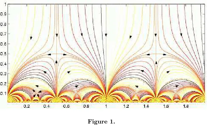
and this is the minimal choice in the sense that it has the fewest possible singular points. The flow generated by (3.10) is shown in Fig. 1, there are fixed points on the real axis at τ =q/p
where the massless dyons have quantum numbers (nm, ne) = (−p, q). Odd p corresponds to attractive fixed points in the IR direction and even p to attractive fixed points in the UV direction (p = 0 corresponds to the original weakly coupled theory, τ = i∞). The repulsive singularities at τ = n+2i withn an odd integer occur for u = 0 and are the quantum vestige of the classical situation were full SU(2) symmetry would be restored.
One point to note is that, since the scaling function (3.10) is symmetric underu→ −u, which is equivalent toτ →τ+ 1, the full symmetry of the scaling flow is slightly larger than Γ(2), it is generated by F2 and T and corresponds to matrices γ such thatc in (2.9) is even. This group is often denoted by Γ0(2).
Observe also that there are semi-circular trajectories linking some of the IR attractive fixed points with odd monopole charge. These can all be obtained from the semi-circular arch linking
τ = 0 and τ = 1 by the action of some γ =
a b c d
∈Γ0(2). Then
τ1 =q1/p1 =γ(0) = b
and
τ2 =q2/p2 =γ(1) = a+b
c+d (3.12)
from which b=±q1,d=±p1 andq2=±(a+b), p2 =±(c+d). Hence
|q2p1−q1p2|= 1, (3.13)
since ad−bc = 1, giving a selection rule for transitions between IR attractive fixed points as the massesu are varied. This is clearly related to the Dirac–Schwinger–Zwanziger quantisation condition (2.5).
When matter in the fundamental representation is included the picture changes in detail, but is similar in structure [5]. In particular different subgroups of Γ(1) appear. To anticipate the notation let Γ0(N)⊂Γ(1) denote the set of matrices with integral entries and unit determinant
γ =
a b c d
such thatc= 0 mod N and let Γ0(N) ⊂Γ(1) denote those with b= 0 mod N.
These are both subgroups of Γ(1): Γ0(N) being generated by T and S−1TNS while Γ0(N) is generated by TN and S−1T S.
Now considerN = 2 supersymmetric SU(2) Yang–Mills theory in 4-dimensional Minkowski space with Nf flavours in the fundamental representation of SU(2). The low energy effective action for 0< Nf <4 was derived in [5] (Nf = 4 is a critical value for which the quantum theory hasβ(τ) = 0 and the theory is conformally invariant). Because matter fields in the fundamental representation of SU(2) can have half-integral electric charges it is convenient to re-scaleτ by a factor of two and define
τ′ = θ
π +
8πi
g2 . (3.14)
Thus
γ(τ) =τ + 1 ⇒ γ(τ′) = 2γ(τ) =τ′+ 2 (3.15)
and
γ(τ) = τ
1−2τ ⇒ γ(τ
′) = 2γ(τ) = τ′
1−τ′, (3.16)
so Γ0(2) acting onτ is equivalent to Γ0(2) acting onτ′.
The quantum modular symmetries of the scaling function acting onτ′ are
Nf = 0, Γ0(2),
Nf = 1, Γ(1),
Nf = 2, Γ0(2), Nf = 3, Γ0(4)
and explicit forms of the corresponding modular β-functions are given in [49]. For Nf = 1 and
Nf = 3 the group is the same as the symmetry group acting on the effective action while for
Figure 2.
4
Duality and the quantum Hall ef fect
Modular symmetry manifests itself in the quantum Hall effect (QHE) in a manner remarkably similar the that of N = 2 supersymmetric Yang–Mills. But while N = 2 supersymmetry is not generally believed to have any direct relevance to the spectrum of elementary particles in Nature, the quantum Hall effect is rooted in experimental data and its supremely rich structure was not anticipated by theorists. The first suggestion that the modular group may be related to the QHE was in [2] but, as we shall see below, the wrong subgroup was identified in this earliest attempt.
The quantum Hall effect is a phenomenon associated with 2-dimensional semiconductors in strong transverse magnetic fields at low temperatures, so that the thermal energy is much less than the cyclotron energy ~ωc, with ωc the cyclotron frequency. It requires pure samples
with high charge carrier mobility µso that the dimensionless productBµ is large. For reviews see e.g. [50,51, 52]. Basically passing a current I through a rectangular 2-dimensional slice of semi-conducting material requires maintaining a voltage parallel to the current (the longitudinal voltage VL). The presence of a magnetic field B normal to the sample then generates a trans-verse voltage (the Hall voltage VH). Two independent conductivities can therefore be defined: a longitudinal, or Ohmic, conductivityσLand a transverse, or Hall, conductivityσH, along with the associated resistivities, ρL andρH. The classical Hall relation is
B =enρH ⇒ σHB=−Je0 (4.1)
(with J0
e =enand nthe density of mobile charge carriers) and σH is inversely proportional to
B at fixedn. In the quantum Hall effectσH is quantised as 1/Bis varied keeping nandT fixed (or varying nkeepingB and T fixed) and increases in a series of sharp steps between very flat plateaux. At the plateaux σL vanishes and it is non-zero only for the transition region between two adjacent plateaux. In 2-dimensions conductivity has dimensions of e2/h and, in the first experiments, [53]σH =ne
2
Figure 3.
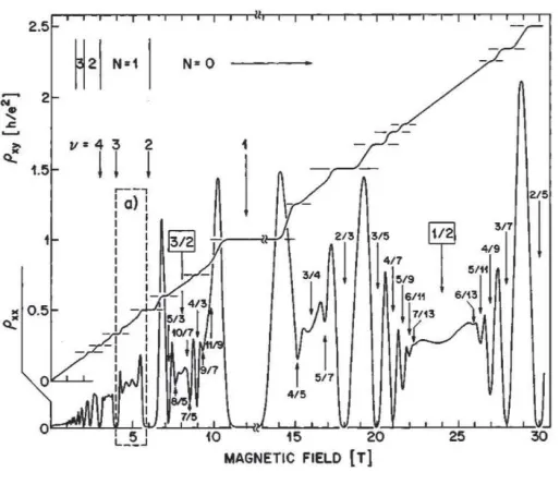
σH = qpe 2
h where p is almost always an odd integer (from now in this section on we shall adopt units in whiche2/h= 1). The different quantum Hall plateaux are interpreted as being different phases of a 2-dimensional electron gas and transitions between the phases can be induced by varying the external magnetic field, keeping the charge carrier density constant. An example of experimental data is shown in Fig. 3, taken from [55], where the Hall resistivity (ρxy) and the Ohmic resistivity (ρxx) for a sample are plotted as functions of the transverse magnetic field, in units ofh/e2. The Hall resistivity is monotonic, showing a series of steps or plateaux, while the Ohmic resistivity shows a series of oscillations with deep minima, essentially zero, when ρxy is at a plateaux, and a series of peaks between the Hall plateaux.
Conductivity is actually a tensor
Ji =σijEj (4.2)
withσxx andσyy the longitudinal conductivities in thexandydirections andσxy =−σyx=σH the Hall conductivity associated with the magnetic field (for an elementary discussion of the Hall effect see [56]). From now on we shall assume an isotropic medium with σxx =σyy =σL. Using complex co¨ordinates z = x+iy the conductivity tensor for an isotropic 2-dimensional medium can be described by a single complex conductivity
σ :=σH +iσL. (4.3)
Note that Ohmic conductivities must be positive for stability reasons, so σ is restricted to the upper half-complex plane. The resistivity tensor is the inverse of the conductivity matrix, in complex notation ρH +iρL=ρ=−1/σ.
In [17] it was argued that the following transformations
T :σ → σ+ 1 and F2:σ → σ
1−2σ (4.4)
map between different quantum Hall phases of a spin polarised sample. These transformations are known as the Law of Corresponding States for the quantum Hall effect7.
7
The T transformation is interpreted as being due to shifting Landau levels by one, e.g. by varying the magnetic field keeping nfixed. The philosophy here is that a full Landau level is essentially inert and does not affect the dynamics of quasi-particles in higher Landau levels. The number of filled Landau levels is the integer part of the filling factorν = nh
eB and quasi-particles in a partially filled Landau leveln, withna non-negative integer, and filling factorν=n+δν, 0 ≤ δν < 1, will have similar dynamics to situations with the same δν and any other n. In particular n → n+ 1 should be a symmetry of the quasi-particle dynamics. The situation here is similar to that of the periodic table of the elements were fully filled electron shells are essentially inert and do not affect the dynamics of electrons in higher shells – noble gases would then correspond to exactly filled Landau levels (the quantum Hall effect is in better shape than the periodic table of the elements however because all Landau levels have the same degeneracy whereas different electron shells have different degeneracies). Of course this assumes that there is no inter-level mixing by perturbations and this can never really be true for all n. To achieve large nfor a fixed carrier density n, for example, requires small B and eventuallyB will be so small that that the inter-level gap, which is proportional toB, will no longer be large compared to thermal energies and/or Coulomb energies.
The F transformation, known as flux-attachment, was used by Jain [57, 58], though only for Hall plateaux σL = 0, as a mapping between ground state wave-functions. Jain’s mapping was associated with modular symmetry in [59] and with modular transformations of partition functions in [60]. It is related to the composite fermion picture of the QHE [51,61,62,63] where the effective mesoscopic degrees of freedom are fermionic particles bound to an even number of magnetic flux units, the operation F2 attaches two units of flux to each composite fermion, maintaining their fermionic nature, in a manner that will be described in more detail below.
The response functions (i.e. the conductivities) in a low temperature 2-dimensional system can be obtained from a 2+1-dimensional field theory by integrating out all the microscopic physics associated with particles and/or holes and incorporating their contribution to the macroscopic physics into effective coupling constants. The classical Hall relation (4.1) can be derived from
Leff[A0, Je0] =σHA0B+A0Je0, (4.5)
where J0
e is the charge density of mobile charges only, not including the positive neutralising background of the ions. The co-variant version of this is
Leff[A, Je] = σH
2 ǫ µνρA
µ∂νAρ+AµJeµ, (4.6)
where µ, ν, ρ = 0,1,2 label 2+1 dimensional coordinates. In linear response theory the Hall conductivity here would be considered to be a response function, the response of the system to an externally applied electromagnetic field. Ohmic conductivity can be included by working in Fourier space (ω,p) and introducing a frequency dependent electric permittivity. In a conductor the infinite wavelength electric permittivity has a pole at zero frequency, in a Laurent expansion
ǫ(ω,0) =−iσL
ω +· · · , (4.7)
and all of the microscopic physics can be incorporated into response functions that modify the effective action for the electromagnetic field. In Fourier space, in the infinite wavelength, low-frequency limit, the modification is
e
Leff[A]≈ iσL
4ωF 2+σH
4 ǫ µνρA
µFνρ, (4.8)
where F2 = F
xi
xj
xi- xj
φij
O
Figure 4.
in the sample, from which response functions can be read off. The most relevant correction, in the renormalisation group sense, is the Chern–Simons term in (4.8). Naively assuming that there are no large anomalous dimensions arising from integrating out the microscopic degrees of freedom, the next most relevant term would be the usual Maxwell term. It is an assumption of the analysis in [17] that other terms, higher order inF and its derivatives, are not relevant.
Note that the right hand side of (4.8) is not real, an indication of the dissipative nature of Ohmic resistance, and non-local in time, again a feature of a conducting medium. Also we have used a relativistic notation and F2 should really be split into E·E and B·B with different coefficients (response functions). In the p = 0, low-frequency limit of a conductor however, both response functions behave as 1/ω, the ratio is a constant and a relativistic notation can be used8. Chern–Simons theories of the QHE have been considered by a number of authors [17,64,65,66,67,68,69,70]. The presence of theF2 term has been analysed from the general point of view of 3-dimensional conformal field theory in [71,72,73,74].
For strong magnetic fields however (4.8) is not small and linear response theory cannot be trusted. This problem can be evaded by introducing what is called the “statistical gauge field”, aµ, [63,65,75,76], and then following the analysis of [17]. Consider a sample of material with N charge carriers with wave-function Ψ(x1, . . . ,xN). Perform a gauge transformation
Ψ(x1, . . . ,xN) → Ψ′(x1, . . . ,xN) =e iϑ(P
i<j
φij)
Ψ(x1, . . . ,xN), (4.9)
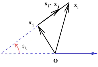
where φij is the angle related to the positions of particle i and particle j as shown in Fig. 4, in terms of complex coordinates, z = x+iy, eiφij = zi−zj
|zi−zj|. ϑ is a constant parameter and
can change the statistics of the particles: for example if the particles are fermions, so that Ψ is anti-symmetric under interchange of any two particles iandj, i.e. when φij →φij+π, then Ψ′ is again anti-symmetric if ϑ= 2k is an even integer, Ψ′ becomes symmetric ifϑ= 2k+ 1 is an odd integer.
For co-variant derivatives, (−i~∇ −eA)µ acting on Ψ becomes (−i~∇ −eA−a)µ acting
on Ψ′ under (4.9) where
aα(xi) =~ϑ X
j6=i
∇(αi)φij =−~ϑ X
j6=i
ǫαβ
(xi−xj)β
|xi−xj|2
, (α, β = 1,2). (4.10)
As long as the particles have a repulsive core, so xi 6= xj for i 6= j, the potential a is a pure gauge, but if the particles can coincide there is a vortex singularity inaand
ǫβα∇(βi)aα(xi) =hϑ X
j
δ(2)(xi−xj)→hϑn(xi), (4.11)
8
the last expression being the continuum limit of the discrete particle distribution. The statistical gauge field aµ was introduced in the context of “anyons” in [65, 75]. Its relation with the charge carrier density (4.11) was pointed out in [76], where similarities between the statistics parameterϑand the vacuum angle QCD were noted and it was observed the binding of vortices to particles is a 2+1-dimensional version of ’t Hooft’s notion of oblique confinement in QCD [77], in which a condensate of composite objects occurs.
The constraint (4.11) can be encoded into the dynamics, by introducing a Lagrange multip-liera0, and then made co-variant by modifying (4.6) to read
Lef f[A, a, Je] = coefficient of the AµChern–Simons term has been changed fromσH to a new parameters, this is because quantum effects modify the Hall coefficient and identifying σH with sis premature at this stage. Following [17] it is now argued that integrating out Ψ′ in (4.12) to get an effective
action forA and acan only produce terms that depend on the combination A′ :=A+a/e and gauge invariance restricts the allowed terms9. Define the field strength forA′ as usual
Fµν′ =∂µA′ν −∂νA′µ (4.13)
and that of aas
fµν =∂µaν −∂νaµ. (4.14)
Then the effective action, in Fourier space in the long-wavelength p = 0 limit, will be of the form
where the response functions ΠL and ΠH cannot be calculated but are assumed to give con-ductivities in the ω → 0 limit, i.e. it is assumed that ΠL has a pole while ΠH is finite at
ω = 0,
iωΠL(ω) −→
ω→0 σL, ΠH(ω) ω−→→0 σH. (4.16)
Integrating out Ψ′ will in general produce many more terms in the effective action than shown in (4.15), higher order powers inF′ and its derivatives, with unknown coefficients, but it is an assumption of the analysis that these are less relevant, in the renormalisation group sense, than the ΠL and ΠH terms exhibited here. This does require a leap of faith however – while it is certain that there are no anomalous dimensions associated with the Chern–Simons term,ǫA′F′
since it is topological, it is by no means obvious that integration of Ψ′ will not produce large
anomalous dimensions associated with operators like (F′2)2, for example, that might render them more relevant that F′2. It is an assumption in [17] that this does not happen. Note however that it has been assumed that there is a large anomalous dimension associate with F′2 – this operator is not naively marginal in 2+1-dimensions, but the assumption of a pole in ΠL renders it marginal. The effective action (4.15) is actually conformal [71]. One further modification of the effective action used in [17] is to allow for a change in the effective charge of the matter fields Ψ′,e∗=ηe. This is easily incorporated into (4.15) by redefiningA′ to be A′ =ηA+a/e
everywhere (the units are not affected, we still have h=e2).
9
TheF2andT transformations in (4.4) can now be derived by integratingaout of the effective action (4.15), which is quadratic in a and so the integration is Gaussian. This leads to a new effective action forA alone, with different conductivities,
e
The analysis of was taken further in [81] and extended beyond the regime of linear response in [82].
Note that detγ = 1 so the most general transformation, for arbitrarys,ϑandη, is an element of Sl(2;R). However a general element is not a symmetry, for example if ϑ is not an integer then the two conductivities describe charge carriers which are anyons with different statistics. Also ifϑ is an odd integer we have mapped between bosonic and fermionic charge carriers and this is not a symmetry, though this was the map described in the analysis in [17] where σ was associated with a bosonic system, which could form a Bose condensation, andσ′ was associated with a quantum Hall system with fermionic charge carriers (there is no suggestion here that a supersymmetric theory necessarily underlies the quantum Hall effect).
Quantum mechanics requires that the parameters η, s and ϑ in (4.19) must necessarily be quantised for the map to be a symmetry. For example η = 1, when the charge carriers are pseudo-particles with e∗ =e, withϑ= 0 gives
and we only expect this to be a symmetry when s is an integer (Landau level addition). In particular γ(1,1,0) gives the T transformation of (4.4). The flux attachment transformation,
F2 in (4.4), follows from the fact that ϑ= 2k should be a symmetry for any integral k, with
We can now map between different Hall plateaux by combining the operations of adding statistical flux and Landau level addition. For example if we start from a plateau with σ = 1 and perform a (singular) gauge transformation with ϑ= 2, which isF−2, then we transform to a new phase withσ = 1/3.
Note that a general transformation requiresη6= 1, although it is always rational. For example the Jain series of fractional quantum Hall states10 can be generated by starting fromσ = 0 and
mapping to Landau levelqusingTq, whereq is a positive integer. Now add 2kunits of statistical flux using F−2k, the resulting transformation is
F−2kTq=
The new conductivity has
σ′ = q
p with p= 2kq+ 1 and η =
1
p,
so the pseudo-particles carry not only 2k vortices of statistical flux but also electric charge
e∗= e
p
with p odd, i.e. fractional charge. This is precisely analogous to the Witten effect described in Section 2. Fractional charges of e/3 for q = k = 1 were predicted in [78] and have been confirmed by experiment [79,80].
The model of the Hall plateaux espoused in [17] is that one has charge carriers which are fermions (electrons or holes) interacting strongly with the external field. By attaching an odd number 2k+ 1 of statistical flux units to each fermion the resulting composite particles are bosons. By choosingkappropriately it can be arranged that the effect of the external magnetic field is almost cancelled by the statistical gauge field and the composite bosons behave almost as free particles. Being bosons they can condense to form a superconducting phase, with a mass gap, and this explains the stability of the quantum Hall plateaux for the original fermions. This map between bosons and fermions is of course not a symmetry, nevertheless it is a useful way of looking at the physics. An alternative view is Jain’s composite fermion picture [51,61,62,63], which is a symmetry. Both the composite fermion and the composite boson picture are useful, but in either case fermions lie at the heart of the physics, as indicated by the antisymmetry of the Laughlin ground state wave-functions.
The transformations (4.4) acting on the complex conductivity map between different quantum Hall phases, clearly they generate the group Γ0(2). As mentioned above the relevance of the modular group to the QHE was anticipated by Wilczek and Shapere [2], though these authors focused on a different subgroup of Γ(1), one generated by
S :σ→ −1/σ and T2 :σ→σ+ 2 (4.22)
(denoted by Γθ here and by Γ1,2 in [2]) and the experimental data on the QHE do not bear this out. For example Γθ has a fixed point atσ =ithere is no such fixed point in the experimental data for the quantum Hall effect. We shall return to Γθ below in the context of 2-dimensional superconductors. L¨utken and Ross [13] observed, even before [17], that the quantum Hall phase diagram in the complex conductivity plane bore a striking resemblance to the structure of moduli space in string theory, at least for toroidal geometry, and postulated that Γ(1) was relevant to the quantum Hall effect. In [14, 15, 16] the subgroup Γ0(2) was identified as being one that preserves the parity of the denominator and therefore likely to be associated with the robustness of odd denominators in the experimental data.
Among the assumptions that go into the derivation of (4.4) from (4.8) are that the tempera-ture is sufficiently low and that the sample is sufficiently pure, but unfortunately the analyses in [13,14,17,82] are unable to quantify exactly what “sufficiently” means. Basically one must simply assume that (4.8) contains the most relevant terms for obtaining the long wavelength, low frequency response functions, but obviously this is not always true even at the lowest tem-peratures, for example it is believed that, at zero temperature, a Wigner crystal will form for filling fractions below about 1/7 and (4.8), being rotationally invariant, cannot allow for this11.
Of course Γ0(2) is not a symmetry of all of the physics, after all the conductivities differ on different plateaux, nevertheless it is a symmetry of some physical properties. The derivation of the Γ0(2) action in [17] required performing a Gaussian integral about a fixed background,
11
different backgrounds give different initial conductivities, but in each case the dynamics con-tributing to the fluctuations are the same and the dynamics of the final system have the same form as that of the initial one. This motivates the suggestion [84, 85, 86, 87] that the scaling flow, which is governed by the fluctuations, should commute with Γ0(2), i.e. although Γ0(2) is not a symmetry of all the physics it is a symmetry of the scaling flow. Physically the scaling flow of the QHE can be viewed as arising from changing the electron coherence length l, e.g. by varying the temperature T with l(T) a monotonic function of T [88, 89]. Define a scaling function by
Σ(σ,σ¯) :=ldσ dl.
In general one expectsσ to depend on various parameters, such as the temperature T, the external fieldB, the charge carrier densitynand the impurity densitynI. Ifnand nI are fixed thenσ(B, T) becomes a function ofB andT only. The scaling hypothesis of [89] suggests that, at low temperatures, σ becomes a function of a single scaling variable.
Now for anyγ ∈Γ(1),γ(σ) = cσaσ++db withad−bc= 1, so
Σ γ(σ), γ(¯σ)= 1
(cσ+d)2Σ(σ,¯σ),
this is always true, by construction, and does not represent a symmetry.
Demanding that Γ0(2) is a symmetry of the QHE flow we immediately get very strong predictions concerning quantum Hall transitions. Firstly one can show that any fixed point of Γ0(2), withσxx >0, must be fixed point of the scaling flow (though notvice versa), [84]. To see this assume that the scaling flow commutes with the action of Γ0(2) and let σ∗ be a fixed
point of Γ0(2), i.e. there exists aγ ∈Γ0(2) such that γ(σ∗) =σ∗. Ifσ∗ were not a scaling fixed
point, we could move to an infinitesimally close pointδf(σ∗)6=σ∗ with an infinitesimal scaling
transformation,δf. Assumingγ δf(σ∗)
=δf γ(σ∗)) =δf(σ∗) then implies thatδf(σ∗) is also
left invariant by γ. But, for ℑσ >0 and finite, the fixed points of Γ0(2) are isolated and there is no other fixed point of Γ0(2) infinitesimally close to σ∗. Hence δf(σ∗) = σ∗ and σ∗ must
be a scaling fixed point. Fixed points σ∗ of Γ0(2) withℑσ >0 are easily found by solving the equation γ(σ∗) = σ∗: there is none with ℑσ > 1/2: there is one at σ∗ = 1+2i, indeed a series
with σ∗ = n+2i for all integral n, and of course the images of these under Γ0(2), leading to a fractal structure as one approaches ℑσ = 0. Many of these fixed points have been seen in experiments [84].
Experiments show that fixed points between plateaux correspond to second order phase tran-sitions between two quantum Hall phases and modular symmetry implies that scaling exponents should be the same at each fixed point, a phenomenon known as super-universality [90, 91]. The idea here is that the transition between two quantum Hall plateaux is a quantum phase transition [92] and, at low temperatures, σ becomes a function of the single scaling variable ∆TBκ
with a scaling exponentκ, where ∆B =B−Bc withBc the magnetic field at the critical point. While there is evidence for super-universality withκ≈0.44 [90,93], there are some experiments which seem to violate it [94]. This may be due to the suggestion that there exists a marginal operator at the critical point [95], but an alternative explanation, that the scaling function might be a modular form, is proposed in [96].
A second striking consequence of Γ0(2) symmetry of the scaling flow is a selection rule for quantum Hall transitions which can be derived in exactly the same way as in the discussion around (3.13) in Section 3. Given that the integer transition σ: 2→1 is observed we conclude that γ(2) → γ(1) should also be possible. Let γ(1) = q1
p1 and γ(2) = q2
σ
0 1
Figure 5.
mutually prime, as are q2 andp2. Then, withγ =
a b c d
,
q1 p1
= a+b
c+d and
q2 p2
= 2a+b
2c+d (4.23)
so,
q1 =±(a+b), p1=±(c+d), q2 =±(2a+b) and p2 =±(2c+d).
Since ad−bc= 1 we obtain the selection rule [84]
|q2p1−q1p2|= 1. (4.24)
This selection rule is well borne out by the experimental data in Fig. 3. In spin-split samples any two adjacent well-formed plateaux, with no unresolved sub-structure between them, obey this rule12.
If we further assume that theonlyfixed points of the scaling flow are the fixed points of Γ0(2) then, with a few extra reasonable assumptions, the topology of the flow diagram is completely determined and it is exactly the same as in Fig. 1 for N = 2 SUSY. The whole upper-half plane can be covered by starting with the infinite strip of width 1 above the semi-circular arch spanning 0 and 1 in Fig. 1 (called the fundamental domain of Γ0(2) and shown in Fig. 5, [47]) and acting on it with elements of Γ0(2). IR fixed points haveτ =q/pcorresponding to fermionic charge carriers which can be viewed, by turning [17] around, as bosons withpunits of statistical flux attached, where p is odd.
Guided by experiment, the reasonable assumptions are [96]:
• Rational numbers q/p with oddp are attractive, since they are experimentally so stable;
• The flow comes down vertically from the points at σ = σH +i∞ i.e. that σH does not flow at high temperatures (weak coupling [96,97])
then the topology forces the fixed points with ℑσ > 0 to be saddle points and the only flow possible is compatible with the topology of Fig.1. The precise form of the flow in Fig.1can be deformed, but the fixed points cannot be moved.
12
Figure 6.
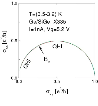
An even stronger statement can be made with one further assumption. When a system is symmetric under particle-hole interchange one has symmetry under change of the sign of σH, which isσ→1−σ¯ for the complex conductivity. This puts a reality condition on Σ(σ,σ¯) which, combined with the mathematical properties of invariant functions of Γ0(2), can be used to show that the boundary of the fundamental domain in Fig.5, and its images under Γ0(2) must always be flow lines, [98]. Any deformation of Fig.1 must therefore leave invariant not only the fixed points but also the vertical lines above integers on the real axis and the semi-circles spanning rational numbers on the real line with odd denominators, (as well as the images of these under Γ0(2)) – only the specific shape of the flow lines inside the fundamental domain, and their images under Γ0(2), can be deformed. In particular Γ0(2) symmetry provides a remarkably robust derivation of the well-established experimental semi-circle law. In many experiments the transition between two plateaux does follow a semi-circle in the upper-half complex conductivity plane to a very high degree of accuracy, Fig. 6 for example is taken from [99]. (Note however that the critical point, as indicated byBc in Fig.6, is not atσ= (1 +i)/2 as would be predicted by Γ0(2) symmetry. This will be discussed below.) The scaling hypothesis of [89,90] described above suggests that, at low temperatures,σ becomes a function of the scaling variable ∆TBκ and
the flow is then forced onto one of these semi-circles as T →0. At a microscopic level the semi-circle law has been derived in one specific model [100, 101], but modular symmetry provides a very robust derivation, [98], valid for any model which satisfies the above assumptions, and is therefore much more general than any specific model. Any deviation from a semi-circular transition is an experimental signal that the sample under investigation is not symmetric under particle-hole interchange. The general topology of the flow in Fig. 1, at least for the integer QHE, was predicted by Khmel’nitskii [88], though the normalisation of the vertical axis was not determined in that analysis and there was no extension to the fractional case13.
The specific flow for Fig.1 was determined by supplementing the above assumptions with one more condition, that the scaling function Σ(σ) should be a meromorphic function in the argument σ14. This makes Σ(σ) a modular form of weight −2 and the analytic form that approaches the stable fixed points on the real axis most rapidly is then exactly the same as that of N = 2 SUSY Yang–Mills in the previous section, up to an undetermined constant, namely
Σ(σ) = 2
πi
1
ϑ4
3(σ) +ϑ44(σ)
, (4.25)
13
A similar topology appears in the flow of one-dimensional clock models [8], but there is no obvious connection with the modular group in these models.
14
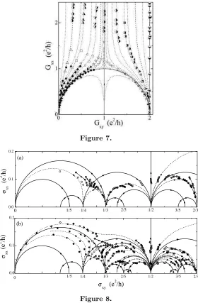
Figure 7.
0.0 0.1 0.2 0.0 0.1 0.2
3/5
0 1/5 1/4 1/3 2/5 1/2 2/3
σxx
(e
2 /h
)
(b) (a)
1/5
0 1/4 1/3 2/5 1/2 3/5 2/3
σxx
(
e
2 /h
)
σxy (e2/h)
Figure 8.
and this gives the flow plotted in Fig. 1. To date there is no physical reason for assuming that Σ should be independent of ¯σ, it is only motivated by mathematical analogy with SUSY Yang– Mills, but it does have the advantage of giving an explicit form for the scaling function that can be visualised. Any deformation away from holomorphicity by including a non-meromorphic component is constrained by the considerations above and cannot change the topology. In fact the flow obtained using the meromorphic ansatz does give remarkably good agreement with experiment and the comparison is plotted in Figs. 7 and 8, taken from [102, 103] (in Fig. 7
the Landau levels are spin-degenerate and this has the effect of doubling the conductivity – see below and footnote 15). Alternative, non-holomorphic forms, have recently been proposed [104,105].
In summary, modular symmetry Γ0(2) applied to the quantum Hall effect for spin-split sam-ples leads to the following predictions:
• Universal critical points are predicted atσ∗ = 12(1 +i) and its images under Γ0(2). Critical exponents must be the same for all fixed points which are related by Γ0(2).
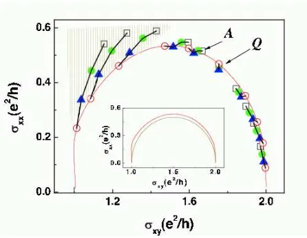
Figure 9.
• Flow in the infrared is towards the real axis, terminating on the real axis at attractive fixed points at odd-denominator fractions. Even-denominator fractions form repulsive fixed points of the flow.
• The selection rule|p1q2−p2q1|= 1 for allowed transition betweenσ =q1/p1andσ =q2/p2.
For QHE samples that are not fully spin polarised one expects that the Landau levels can come in adjacent pairs and T in (4.4) should be replaced byT2, giving the generators of Γ(2) rather than Γ0(2), and this modifies the experimental consequences. Γ(2) actually has no fixed points above the real axis, so one cannot make any predictions about the position of the second order phase transition between two plateaux, but if there is particle-hole symmetry one still has the semi-circle law and the fixed point must lie somewhere on the semi-circle, [106]. An experimental analysis of the relation between modular symmetry and Zeeman splitting is given in [107,108,109] and the results support the interpretation in [106]. Fig.9is reproduced from [109] and represents a sample where the spin splitting is small, significantly less than the Landau level splitting but still non-negligible in the low Landau levels where the magnetic field is large, and Γ0(2) symmetry is broken to Γ(2), so the critical point,Q in the figure, is not at the top of the semi-circle. Nevertheless particle-hole symmetry is obeyed reasonably well, as manifest by the close approximation to a semi-circle. In the same sample, at lower magnetic fields and higher Landau levels the spin-splitting becomes negligible and the sample becomes spin-degenerate. In this situation Γ0(2) symmetry again applies, but with the conductivity doubled because of the spin degeneracy in each Landau level. The critical point in the ν = 2 → ν = 4 transition is indeed at the top of the semi-circle in the conductivity plane, as reported in [109]15. It is
possible that the explanation of the fact that Bc is not at the top of the semi-circle in Fig. 6 is due to the spins being poorly split, but there is another possible interpretation for thisν : 1→0 transition [106]. This particular transition is a vertical line in the complex ρ-plane above the point ρ = 1 and a re-scaling of ρxx can move the critical point, which should be at ρxx = 1 if Γ0(2) symmetry holds, to any value ofρxx and hence to any point on the corresponding semi-circle in the σ-plane. If the determination of the scale of ρxx in [99] has an error then Fig. 6 is still compatible with Γ0(2) symmetry. For the particular case of the ν : 1 → 0 transition any re-scaling ofρxx still gives a semi-circle in theσ-plane, but this is not true for other transitions. The observation that the critical point is not atσ= (3+i)/2 for theν : 2→1 transition in [109], as shown in Fig.9, cannot be explained by a re-scaling of the Ohmic resistivity and therefore is
15
Because of the spin degeneracy the transformations areσ→σ+ 2 andσ→ σ
1−σ, i.e. Γ0(2) acting onσ/2 is
equivalent to Γ0
interpreted as a breaking of Γ0(2) symmetry down to Γ(2) because the Landau levels, while not exactly degenerate, are not well split.
The group Γ(2) was also analysed, from the point of view of its action on ground state wave-functions rather than on complex conductivities, in [110] and on complex conductivities in [111,112,113].
Γ0(2) is the subgroup of the full modular group that is relevant for systems with fermionic charge carriers in a strong perpendicular magnetic field with the spins well split. Building on the work of [17], and following a suggestion in [114], it was shown in [81] that Γ0(2) should be the group relevant to 2-dimensional systems involving spin polarised fermionic quasi-particles while Wilczek and Shapere’s group Γθ should be relevant to 2-dimensional systems involving bosonic quasi-particles. If the effective charge carriers are bosonic, e.g. 2-dimensional superconductors, one can obtain predictions from the fermionic case by using the flux attachment transformation to add an odd number of vortices to the quasi-particles. For the case of a single unit of flux this is equivalent to conjugating Γ0(2) by F =S−1T S. Since F−1F2F =F2 and F−1T F =F−2S the resulting group is generated by S and F2, or equivalently S and T2, and is the group Γθ, [2, 82, 81]. Note that the S transformation in (4.22) requires ϑ = −s = ±η with η → ∞ in (4.19). The fixed point σ =i of S is associated with a phase transition from an insulator to a superconductor [115] and a superconductor would have a double pole in its response function, associated with spontaneous symmetry breaking and requiring a mass termm2A2in the effective action. A direct derivation ofS transformation, in conjunction with particle-hole symmetry, for a 2-dimensional superconductor was given in [116]. Γθ consists of elements γ of the form (2.8) with either a, d both odd and b, c both even, or vice versa. In this case the predictions are different from those of Γ0(2):
• Universal critical points are predicted for the flow at the fixed points for transitions be-tween stable phases,σ∗=iand its images under Γθ16.
• The critical exponents at all fixed points related by Γθ must all be the same.
• Exact flow lines in the σ plane are immediate consequences of Γθ invariance and particle-hole symmetry, [81]. The results are again semi-circles or vertical lines in the σ plane, implying a semi-circle law for these bosonic systems.
• For nonzero magnetic fields the flow as the temperature is reduced is towards the real axis, terminating on the attractive fixed pointsσ =p/q withpq even (as opposed to having q
odd, as was the case for fermions). Fractions with odd pq are repulsive fixed points.
• There is a selection rule that allowed fractions p2/q2 can be obtained from p1/q1 only if |p1q2−p2q1|= 1.
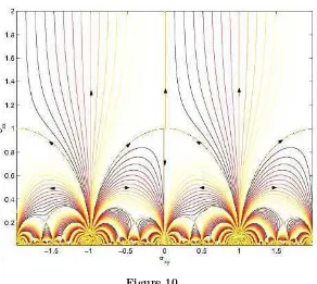
The resulting flow diagram for bosonic systems was first given in [81] and is shown here in Fig. 10. It has a fixed point at σ∗ =i, as predicted by Fisher [115]. To date no 2-dimensional
superconductors have been manufactured with a high enough mobility µ that µB is close to unity for sustainable magnetic fields, but it is predicted in [81] that a hierarchy with the above properties will be observed if such samples are ever manufactured.
5
Conclusions
Modular symmetry is a generalisation of the Dirac quantisation condition for charge in QED. Its mathematical foundation is strongest in supersymmetric systems, in particular supersymmetric
16
This statement is for bosonic charge carriers with the same electric charge as an electron – it becomesσ∗=iq˜
2
Figure 10.
Yang–Mills, but a more realistic system, with a wealth of experimental data to compare with, is the quantum Hall effect.
Effective degrees of freedom are composite objects carrying topologically non-trivial gauge field configurations (monopoles in SUSY Yang–Mills and vortices in the QHE).
For N = 2 SUSY SU(2) Yang–Mills the subgroups of the modular group that are relevant for the scaling modular forms with different numbers of families are
Nf = 0, Γ0(2),
Nf = 1, Γ(1),
Nf = 2, Γ0(2), Nf = 3, Γ0(4).
For the quantum Hall effect the relevant subgroups are
spin-split samples, Γ0(2), spin-degenerate samples, Γ0(2),
intermediate case, Γ(2).
Modular symmetry has important experimental consequences for the quantum Hall effect. The Dirac–Schwinger–Zwanziger quantisation condition manifests itself as a selection rule for transitions between allowed quantum Hall plateaux,
|qp′−q′p|= 1
with Hall conductivities q/p and q′/p′ in spin-split samples (|qp′−q′p|= 2 for spin-degenerate
related to the Witten effect in 3+1-dimensional N = 2 supersymmetric Yang–Mills, where massive excitations can carry electric charge 1/p withp being the monopole number.
For bosonic pseudo-particles the group Γθis predicted to be the relevant group and this gives a suite of predictions similar to the quantum Hall effect but differing in detail, as described in Section 4.
The connection between N = 2 SUSY and the quantum Hall effect that is exposed by modular symmetry is not yet understood, at the moment it is merely at the level of an empirical observation that modular symmetry is relevant to scaling in both these systems. Constructing an explicit map relating one to the other remains an open problem to date. There is a known relation betweenN = 4 SUSY and the quantum Hall effect, [117,118,119], which may prove to be useful starting point, perhaps via SUSY breaking, but since the perturbative β-function for
N = 4 SUSY vanishes there is no clear connection with scaling at present. There are however certain features which bothN = 2 SUSY and the QHE have in common. They all have only two relevant couplings: one, y, associated with the dynamical kinetic term, which must be positive for stability reasons; and one, x, associated with a topological term. These are combined into the complex parameter, τ = x+iy, on the upper half-complex plane on which the modular group, or a subgroup thereof, acts.
An important feature that these systems have in common is the existence of topologically non-trivial field configurations, monopoles in SUSY Yang–Mills and vortices in the QHE, which can bind to the charge carriers to form pseudo-particles carrying magnetic charge: dyons in SUSY Yang–Mills and in the QHE fermions which can be viewed as bosons with an odd number of flux units attached. The rational nature of the attractive fixed points on the real axis q/p is then related to the magnetic charge p. The weak coupling regime, where perturbation theory might be expected to be useful, can be mapped by modular symmetry to the strong coupling regime, where much interesting physics lies.
It seems that modular symmetry is not just an accident of one type of system, or even a family of systems such as supersymmetric field theories, but in fact is a more general phenomenon and it may yet prove even more powerful in understanding the physics of strongly interacting systems.
Acknowledgements
It is a pleasure to thank my long-term collaborator Cliff Burgess for many useful discussions on the quantum Hall effect. This work was partly supported by Enterprise Ireland Basic Research grant SC/2003/415.
References
[1] Dolan B.P., Duality in supersymmetric Yang–Mills and the quantum Hall effect,Modern Phys. Lett. A21
(2006), 1567–1585.
[2] Shapere A., Wilczek F., Self-dual models with theta terms,Nuclear Phys. B320(1989), 669–695. [3] Montonen C., Olive D., Magnetic monopoles as gauge particles,Phys. Lett. B72(1977), 117–120.
[4] Seiberg N., Witten E., Electric-magnetic duality, monopole condensation, and confinement inN= 2 super-symmetric Yang–Mills theory,Nuclear Phys. B 426(1994), 19–53, Erratum,Nuclear Phys. B430(1994), 169–169,hep-th/9407087.
[5] Seiberg N., Witten E., Monopoles, duality and chiral symmetry breaking inN = 2 supersymmetric QCD,
Nuclear Phys. B431(1994), 484–550,hep-th/9408099.
[6] Cardy J.L., Rabinovici E., Phase structure ofZpmodels in the presence of aθparameter,Nuclear Phys. B 205(1982), 1–16.
[7] Cardy J.L., Duality and theθ parameter in Abelian lattice models,Nuclear Phys. B205(1982), 17–26. [8] Asorey M., Esteve J.G., Salas J., Exact renormalization-group analysis of first-order phase transitions in