www.elsevier.nl / locate / econbase
Unemployment insurance benefit levels and consumption
changes
a ,* b,c
Martin Browning , Thomas F. Crossley
a
Institute of Economics, University of Copenhagen, Studiestraede 6, DK-1455 Copenhagen, Denmark
b
Department of Economics, York University, Toronto, Canada c
Centre for Economic Policy Research, Research School of Social Sciences, The Australian National University, Canberra, Australia
Received 1 September 1998; received in revised form 1 December 1999; accepted 1 January 2000
Abstract
We use a Canadian survey of the unemployed to examine how household expenditures after a job loss respond to the level of income replacement provided by UI. We isolate a liquidity constraint or ‘transitory income’ effect from the ‘permanent income’ shock of job loss, and from the costs of working. We find significant effects of varying the replacement ratio among the third of the sample who did not have assets at the job loss. We conclude that the consumption smoothing benefit of UI is concentrated wholly on a sub-group of the unemployed. 2001 Elsevier Science S.A. All rights reserved.
Keywords: Unemployment insurance; Living standards; Consumption; Liquidity constraints
JEL classification: D91; J65
1. Introduction
Should governments provide unemployment insurance and, if so, what should the provisions be? There have been numerous studies of the costs of unemploy-ment insurance (UI) in recent years but fewer attempts to measure the benefits.
*Corresponding author. Tel.:145-35-323-070; fax:145-35-323-064. E-mail address: [email protected] (M. Browning)
Households may benefit from UI in several ways. The ‘consumption smoothing’ benefit of UI is realized by liquidity constrained households that have temporarily low income and are not able to set their current consumption at a level consistent with their expectations of the future. The ‘insurance’ benefit of UI arises because
1
UI, like a progressive tax, reduces the variance of stochastic outcomes. That UI has an ‘insurance’ benefit requires only that households be risk adverse and not otherwise fully insured against idiosyncratic shocks; in particular, borrowing constraints are not a necessary condition. The ‘consumption smoothing’ benefit of
2
UI is often thought to be the most important potential benefit of UI, and it is this benefit which is the focus of this paper.
We use a new Canadian panel data set to examine household expenditure changes across a job loss and how those changes vary with the level of replacement income provided by UI. Household expenditure changes with unemployment confound three things: the costs of working (changes in expendi-ture due to the non-separability of consumption from labor supply), a response to the ‘permanent income’ shock of job loss, and, a response to ‘transitory income’. Responses to transitory income are informative about the ‘consumption smooth-ing’ benefit of UI. Specifically, if households respond to marginal changes in ‘transitory income’ then they are not on their optimal consumption path, and marginal actuarially fair increases in UI replacement income (that increase current income and lower future income) raise household welfare, moving the household towards that optimal path.
The form of our test will be to see if differences in the UI replacement ratio across a sample of households experiencing unemployment correlate with differ-ences in the reported expenditure change from before the beginning of the unemployment spell. There is no variation in labor force status across our sample, so our test is not confounded by non-separability between consumption and labor supply. Consequently, to isolate a ‘transitory response’ the main econometric problem we have is that across our sample the UI replacement ratio is plausibly correlated with the permanent shock from a job loss. To overcome this we use rich controls for the permanent shock. We can also test that we have ‘purged’ the UI benefit of its ‘permanent’ component by performing an exogeneity test using instruments that are based on the ‘quasi-experiment’ afforded by two sets of legislative changes (and one administrative change) to the Canadian UI system over our sample period. These instruments are correlated with the temporary loss of income but not with the permanent shock of job loss.
Of the small literature on the benefits of UI, this paper is most similar to Gruber (1997). Our work differs from Gruber’s in several important ways: we use a different measure of expenditure (total, rather than food), a different source of
1
See for example, Varian (1980). 2
variation in benefits (specific legislative changes rather than state-time variation) and of course a different country (Canada rather than the US) which differs in the parameters of its UI system and in other aspects of its social safety net. In addition, our data are rich enough to allow us to focus attention on particular subsets of households which are likely to be liquidity constrained. Since responses to ‘transitory income’ should only be observed among the liquidity constrained, this focus improves our chance of finding indications of large ‘consumption smoothing’ benefits.
An outline of the paper is as follows. In the next section, we derive our estimating equation from a structural model of inter-temporal utility maximization. The presence of a structural model makes explicit the potential sources of gains from UI. Additionally, the structural model allows us to state explicitly and clearly the conditions that allow us to identify the ‘benefit effect’; that is, the impact of marginal changes in the replacement rate on total expenditure. In Section 3 we introduce the data, the Canadian UI system and the legislative and administrative changes that the data capture.
Section 4 presents our empirical results. Our principal finding is that differences in the replacement ratio have small mean effects on household total expenditures. For example, a 10 percentage point cut in benefit levels (from 60% to 50% replacement, for example) would lead to an average fall of only 0.8% in total expenditure, and the implied cut in expenditures due to a 1 dollar cut in benefits (at the means of the data) is less than 7 cents. This mean effect is somewhat smaller than those reported by Gruber (1997). Although the mean effect is small we show that it is concentrated among a small number of households and that most households would not react to a change in the UI replacement rate. The strongest effect is for households that did not have liquid assets at the job separation; this is consistent with the presence of liquidity constraints. We also find a significant effect for respondents who were married but whose spouse was not employed; this suggests that the presence of a second income facilitates consumption smoothing (although we do not find any significant effect for singles). In Section 5, we discuss possible reasons for the difference between our results and those of Gruber (1997) and summarise what we think are the important implications of our results for policy analysis. In particular, we emphasise that the fact that benefit effects are heterogenous invalidates most analysis which effectively assumes a representative agent.
2. Theory
assigned then we could identify the benefit effect simply by looking at how expenditure changes vary with benefit levels. However, benefits are not randomly assigned and cross sectional variation in benefits is correlated with other determinants of expenditures, which we must control for. Furthermore, we will argue that the cross sectional variation in benefits among our sample of job losers is also correlated with determinants of the change in expenditures, so the fact that we first difference the data does not obviate the need for controls.
To illustrate the biases that would arise from just regressing consumption changes on the replacement rate, consider two variables: ‘earnings on the lost job’ and the agent’s ‘attachment to the labor force’. For the former, it is plausible that high earners experience a larger shock with job loss and have a lower replacement rate (details will be given below). Thus the correlation between consumption changes and the replacement rate partially reflects this effect. The bias from ‘attachment to the labor force’ has the opposite sign since attachment is negatively correlated with the replacement rate but positively correlated with the job loss shock since ‘low attachment’ workers do not experience much of a negative job shock loss. These two examples also illustrate that there may be a bias from ignoring permanent variables and that this bias can be positive or negative.
We begin by considering changes in expenditure around a job separation for an agent who lives alone. We consider a discrete period, single non-durable good model in which new information is only revealed at the end of each period. Consumption in any period takes place before the end of period information is known but after the current period income is revealed. We are considering an agent who suffers a job loss, so let period t be the period before the job separation and period t11 the period after; thus the job separation takes place at the end of period t and may not be fully anticipated in period t.
Let lt be the marginal utility of expenditure in period t; the condition for optimal intertemporal allocation between t and t11 gives that
lt115l 2t ut11 (1)
3
where ut11 is a ‘surprise’ error term which is orthogonal to the information set in time t; it includes the shock from the job loss (and hence is likely to be negative) as well as any other new information that arrives at the end of period t. Thus:
E(ut11uI )t 50 (2)
(where I is the information available at time t). However, our sample below takest only those who experienced a job loss. If this separation is partially unexpected (with respect to the information set at time t) then we have that the expectation of ut11 conditional on I and a separation occurring between t and tt 11 is negative and may be correlated with past information.
3
To formalize this, let the realized shock beD 1L et11if the agent loses their job between periods t and t11 and D 1E et11 otherwise. Thus DL represents the ‘permanent’ shock (the revision to the marginal utility of expenditure) from a job loss. The residual term et11 captures all of the impact of news except for that concerning any job loss. Thus E(et11uI )t 50. Ifpt is the probability of a job loss between t and t11, given the information available at time t, then the latter equation and Eq. (2) give p D 1t L (12pt)D 5E 0. This relationship has a number of implications. Firstly, both of the ‘job’ shocks are zero if there is no uncertainty concerning the job loss (that is, p 5t 0 or 1). Secondly, the two shocks have opposite signs if there is some uncertainty (presumably, DL is negative). Thirdly, the less expected the job separation is, the greater the negative shock associated with a job loss with respect to the shock of keeping the job. Finally, we have the revised version of Eq. (3):
E(ut11uI , Job Loss)t 5 DL. (3)
This captures the important feature of our stochastic specification which is that the Euler equation shock for a selected sample is not necessarily uncorrelated with past information.
There are two sets of correlates for DL. First we have variables that reflect the permanent shock from the job loss; denote these Z where the t subscriptt emphasizes that these variables are known at time t (and some may even be permanent). Examples include the occupation in the lost job, earnings and tenure on that job, the race, age and family situation of the agent and local labour market conditions.
The second set of correlates withDL arise from the possibility of the agent being liquidity constrained. If this is the case then the job loss has a negative impact over and above the permanent shock. More importantly for the purposes at hand, in this case the UI benefit level will enter directly into the determination ofDL and hence into the level of consumption in period t11. Denote any UI benefit received by the agent as Bt11 and pre-separation earnings as Y and define the ‘replacementt ratio’ as at115(Bt11/Y ). As well as the replacement ratio, the level of assets thatt the agent carries forward from period t to period t11 will also affect the level of the liquidity constraint Lagrange multiplier, which we denote m. Denoting asset levels at the beginning of period t11 by At11 we have:
D 5L f(Z ,t m(At11,at11)). (4)
‘benefit effect’. This reflects the impact of transitory changes in income on expenditure.
The job loss function f(Z ,t m(At11,at11)) in Eq. (4) is decreasing in m; this reflects that liquidity constraints make bad shocks even worse. Thus, if the agent is constrained, then increasing the benefit level (and hence the replacement rate) makes the job loss shock less negative. Combining (1), ut115 D 1L et11 and (4) we have the revised Euler equation:
Dlt115 2f(Z ,t m(At11, at11))2et11. (5)
If we parameterize preferences (that is, definelin terms of consumption) and the functions f(.) andm(.) then this gives us an equation for consumption changes that can be estimated from the data. Note that this implicitly invokes the usual Euler equation orthogonality conditions. One major concern in doing this is that we have only two periods. The ‘Chamberlain critique’ points out that the Euler equation orthogonality conditions apply across time and not across agents which invalidates the use of short panels if there are common macro shocks which impact differently on different agents (see Chamberlain (1984) and Browning and Lusardi (1996) for a recent discussion). Here, however, we are conditioning on past levels of Z, so that we only need to invoke the much weaker assumption that, conditional on the Z variables, any common macro shock has the same effect on all agents.
Effectively, then, we identify the benefit effect by assuming that the replacement rate is uncorrelated with the error term in Eq. (5). Even though this is much weaker than assuming that it is uncorrelated with the permanent shock, it is still important to be able to test for the validity of this assumption. To do this involves testing for the exogeneity of the liquidity constraint variables once we have conditioned on the permanent shock variables Z . For this we need variables thatt affect the replacement rate but not the permanent shock; that is instruments for the replacement rate. Since our instruments depend on changes to the Canadian UI system, we leave the details for the empirical section but we emphasize here that we do test the identifying assumption.
Denoting consumption in period t as C we take the following (Frisch ort l-constant) equation for log consumption in period t:
ln Ct5L 1 b 2 lt t (6)
whereLis a constant ‘bliss’ level (which we shall shortly ‘difference away’) such that L.max(ln C ), the variable bt captures the effects of the discounted price
4
level, demographics and discount factors. First differencing and using Eq. (5) we have:
4
ln Ct112ln Ct5(bt112bt)1f(Z ,t m(At11, at11))1et11. (7)
In this equation the first term (bt112bt) captures the effects of the real interest rate, discount rates and changes in the factors that affect preferences. For example, since the agent is employed in period t and unemployed in period t11 one element of this term allows for the cost of going to work which has a negative impact on desired consumption growth. Since there is no variation in this in our data this is absorbed into any constant in f(.). Before discussing the parame-terisation of f(.) we need to take account of two other important features of the environment.
The first issue is that most of our sample of unemployed persons (hereinafter, ‘respondents’) live with other people. The impact of the job separation on household consumption depends on what proportion of pre-separation household income was from the respondent’s earnings. Fairly obviously, if the job lost only accounted for a small fraction of household income we should not expect much of an impact, whatever the replacement ratio. The actual replacement rate we defined above (at11) must be modified to take this into account. From the data we can construct the ratio of the respondent’s pre-separation earnings to pre-separation household income, call this the ‘importance of the respondent’s earnings’. Then define an ‘importance adjusted replacement ratio’, r, by:
r 5(at1121)*(importance of the respondent’s earnings). (8)
This variable is always negative and is close to zero if the replacement ratio is close to unity or if the respondent’s pre-separation earnings were relatively unimportant for the household. It is bounded below by minus unity which represents the case where the respondent’s earnings was the only source of income and this is not replaced at all.
The second feature that we must take account of is that the effects of changing the benefit may be heterogeneous. We have already discussed the case of being liquidity constrained, but there may also be other observable modifiers of the benefit effect. For example, in Canada there is a Social Assistance (or ‘welfare’)
5 scheme which provides a transfer to households that have low income. For households in receipt of Social Assistance, as UI benefits fall, so Social Assistance benefits rise on a one-for-one basis. Thus, a reduction in UI benefits for those who receive Social Assistance will have no effect on current income and we should not observe any benefit effect for the poorest households. It may also be that the labour force status of the respondent’s spouse (if married) will modify the effects of the benefit. We denote the variables that are potential (observable) modifiers of the benefit effect by X, where this may include indicators of being liquidity
5
constrained, being eligible for Social Assistance, having an employed spouse and interactions between these variables; more details are given in the empirical section.
Adopting a linear form for f() andm() we have the following version of Eq. (7):
9
ln Ct112ln Ct5Zta 1 r*X9g 1 et11. (9)
In our empirical work the variables in X are a subset of the controls Z, so that in every case the specification contains levels of these variables as well as their interaction with the benefit variable. The parametersg capture the effects of the adjusted replacement ratio on consumption changes for the different groups in X.
3. Data and institutional environment
The empirical results reported in this paper are based on several legislative changes to the Canadian UI system, and a new panel data set which was created to study those changes. Before April 1993 workers who had a minimum number of weeks of work in the year before a job separation were entitled to UI benefits for a period that could be as long as 1 year. The exact number of weeks to qualify for UI and the weeks of entitlement depended on the local unemployment rate and ranged from 10 to 20 weeks of work to qualify and between 30 and 52 weeks of entitlement. The benefit paid was 60% of pre-separation earnings up to a maximum insurable earnings of $745 per week (for a maximum benefit of $447
6
per week). All those who had a job separation and who met the entitlement qualification were eligible for UI but ‘quitters’ were penalized by a 7 to 12-week waiting period. In April 1993 a series of changes were made to this system. The most important was a reduction in the replacement ratio from 60% to 57% (with a commensurate reduction in the maximum benefit to $425) and the disentitlement of ‘quitters’. A second set of changes came into effect in April and July of 1994. Firstly, the statutory rate was further reduced from 57% to 55%. Secondly, the minimum number of weeks worked in the previous year increased from 10 to 12 weeks in high unemployment regions. Thirdly, the duration of benefits was decreased for any given number of weeks of work in the year prior to the job loss. Finally, individuals with dependents and incomes below $340 per week would receive a 60% statutory replacement rate.
To evaluate the impact of the 1993 changes, a survey of about 11,000 people who had a job separation in February and May of 1993 was conducted by Human Resources Development Canada (HRDC). This survey is known as the Canadian Out of Employment Panel (COEP). Each respondent was interviewed three times,
6
at about 26, 39 and 60 weeks after the job separation. Each interview was conducted over the telephone and took an average of 25 min. Although it would have been desirable to have the first interview at a date closer to the job separation this was not possible since the administrative records that form the sampling frame do not become available until some months after the job separation. This long interval between the job separation and the first interview is the price we have to pay if we wish to sample only those who started an unemployment spell. To evaluate the impact of the 1994 changes, HRDC then commissioned a second survey of about 8000 individuals who separated from a job in February and May of 1995. The survey instrument was refined (and slightly expanded) for this second survey but care was taken to insure backwards comparability. In addition, the third interview was dropped.
To construct the sample used in this paper we began by restricting attention to respondents between the ages of 20 and 60 who lost their job either because of a ‘shortage of work’ (‘laid off’) or because they quit (other than to take another job) or were ‘dismissed with cause’. The main exclusions here are those who left due to illness and those on maternity leave. We also excluded unmarried respondents living with a parent or with unrelated adults. Preliminary analysis indicated that the quality of the responses to the household income and expenditure questions was very poor among these individuals. From the remaining observations we identified a sample of 5318 respondents who were unemployed at the first interview. We next selected those still in the first spell of unemployment; this left 3327 respondents. Thus all those in our sample have been continuously un-employed for about half a year. We then dropped 487 respondents for whom the change in expenditure information was missing. Then we excluded those who had changes in total expenditure that indicated that their current total expenditure was more than double or less than one half of their previous total expenditure. This left a sub-sample of 2617 people. Even for this group some variables are missing so that the final sample size is 1805 respondents.
In this paper we use only information from the first interview of the COEP. In this first wave, a wide range of questions was asked including questions on the pre-separation job; labor market activity in the period between the job separation and the interview; job search details; the activities of other household members; income; expenditure and assets. To the survey data we are able to match several kinds of administrative data for each respondent (and their spouses) covering up to 5 years prior to the survey year.
expenditures, we construct a variable that gives the proportional change in total expenditure from before the job separation to the interview date almost half a year later:
Ct112Ct ]]]
Dln Ct115 C . (10)
t11
Note that this is slightly different from the usual construction in that we divide by the (observed) current level, rather than the lagged (unobserved) level. This is the
7
‘left hand side’ variable of this paper. Among our sample of unemployed respondents the mean consumption fall (as defined above) was 14%. Some 10% of the sample reported falls of 50% of the current level (equivalently, 33% of the lagged level) or more, while more than a quarter reported no change or consumption growth.
The benefit variable we use is the ‘importance adjusted replacement ratio’ variable defined in Eq. (8). The replacement ratio used to calculate this quantity is the ratio of UI benefits currently received relative to the self-reported net-of-tax earnings on the lost job. The UI benefit is derived from administrative records and is believed to be very accurate. Since UI benefits are taxable it is adjusted to a net figure using the respondent’s average UI tax rate for the survey year. The self-reported earnings figure is subject to noise, both because of reporting errors and because the reporting period (hourly, weekly etc.) is not completely clear in
8
every case. The distribution of the replacement ratio is bi-modal with modes at zero (with 22% having no benefit) and at the administrative value of about 60%. The mean is 0.48 and the interquartile range 0.36 to 0.68. For those above the maximum insurable earnings, the actual replacement rate will of course be less than the statutory rate. The actual replacement ratio can exceed the statutory rate if workers earn less per week in the period just before the job separation (to which the earnings question refers) than the average in the 20 weeks before the job loss that are used to calculate the administrative entitlement. Differential tax treatment of benefits and income can also lead to an actual replacement rate which exceeds the statutory value. Our measure of ‘importance’ has a mean of 0.47 and an inter-quartile range of 0.24 to 0.74.
Together, the 1993 and 1995 COEP surveys capture substantial legislative variation in the parameters of the Canadian UI system. In addition, there was some administrative variation in the system during the time period captured by the data. In particular, the maximum level of insurable earnings was increased annually by a formula that substantially outpaced inflation. For individuals above the maximum insurable earnings, these increases more than offset the cuts to the statutory
7
Unfortunately, we cannot construct a similar variable for particular categories of expenditure because the relevant ‘change’ information was not collected.
8
replacement rate so that the real value of benefits increased for high wage workers. The period of 1993 to 1995 was one of slowly improving labor market conditions in Canada (for example, the aggregate unemployment rate fell from 11.2 to 9.5%). Against this background our data capture changes in the UI system that for some individuals increased its generosity (the increase in the maximum insurable earnings and the introduction of the ‘dependents’ rate) while for other individuals the program became less generous (the cuts to the standard statutory rate, the disentitlement of quitters, the decreased weeks of benefit for weeks of work and the increase in the weeks of work required to qualify for benefits).
In addition to the expenditure and benefit variables, we also employ extensive controls for the permanent shock of job loss, demographics and other determinants of expenditures. These controls are based on both the COEP survey responses and administrative data and are detailed in Appendix A.
4. Results
We now turn to our empirical results. We begin by estimating average responses of the expenditure change to the replacement rate for our entire sample. This provides a base case and is comparable to the equation estimated by Gruber (1997).
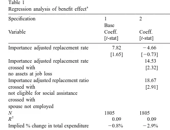
In column 1 of Table 1 we present OLS estimates from the regression of the proportional change in expenditures on our ‘permanent’ controls and the adjusted replacement ratio; only the latter is reported in Table 1. The controls include demographics, household type, regional and seasonal variation, non-wage charac-teristics of the job that ended, measures of the household’s financial resources prior to the job loss, the importance of the respondent’s earnings for pre-separation household income and polynomials in the logarithm of monthly earnings in the lost job and the log of monthly total earnings in previous years (see Appendix A for a complete listing of these variables). The coefficient estimate in column 1 of Table 1 would indicate that for a household in which the respondent’s earnings were the only source of income (‘importance’51) a change in the replacement
9
ratio from 60% to 50% would lead to a 0.8% fall in expenditures. Since a cut in the replacement rate from 60% to 50% represents a cut in the benefit paid of 17% this gives an elasticity of expenditure with respect to the benefit of (0.8 / 17)50.05. We can also calculate the implied cut in total expenditures from a 1 dollar cut in benefits. For a household in which the respondent’s earnings were the only source of income and with sample mean current expenditure level and lost earnings, this number is $0.065. This is a very small effect. However, this is a mean effect and
9
Table 1 Importance adjusted replacement rate 7.82 24.66
[1.65] [20.73]
Importance adjusted replacement rate 14.53 11.55
crossed with [2.32] [2.42]
no assets at job loss
Importance adjusted replacement ratio 18.67 17.71
crossed with [2.91] [2.82]
Implied % change in total expenditure 20.8% 22.9% 22.9% from a 10 point cut in the replacement
rate for importance51
Implied $ change in total expenditure 0.065 0.25 0.26 from a 1$ cut in benefit for
importance51, importance adjusted replacement rate, X are modifiers of the benefit effect, and Z are controls for the demographic determinants of expenditure and for the ‘permanent’ shock of job loss. The controls in Z include: demographics, household type, regional and seasonal variation, non-wage job characteristics, financial resources prior to the job loss, a polynomial in ln(earnings in the lost job), ln(earnings in from previous years). Full results available from the authors.
for all the reasons discussed in the Theory section we might expect the effect to be heterogeneous. Before turning to that issue we consider issues of endogeneity and sample selection.
The validity of our interpretation of the coefficients on the benefit variables rests on the latter reflecting only transitory changes and being uncorrelated with the permanent shock of job loss. Furthermore, our sample is selected on having an unemployment spell of at least 6 months. We have controlled for various correlates of the permanent shock associated with a job loss, such as being a seasonal worker or having high income. In addition to absorbing the permanent shock, this rich set of covariates should also control for many of the differences between our selected sample and separations as a whole.
dummy variable for having no UI benefit. This variable captures a discontinuity at zero. The ‘transitory’ income effects of varying the replacement rate should be continuous but a discontinuity at zero might be generated by ‘permanent income’ effects. To see why, note that those with a positive benefit but a low replacement ratio had high earnings and hence a big permanent shock of job loss. Those with no benefit almost all have less than the required weeks of prior work to qualify for benefits. Consequently they have low attachment to the work force and the job loss represents a relatively smaller permanent shock. The significance of the ‘no benefit’ variable thus provides a first check on whether we have controlled adequately for the permanent shock. The coefficient on this ‘no benefit’ variable is insignificant (a t-value of 0.042) which indicates that we are identifying a genuine transitory benefit effect with the continuous replacement rate variable.
Our second test is a variant of the familiar Durbin–Wu–Hausman test, and tests the adequacy of our controls both with respect to exogeneity of the benefit variables and with respect to sample selection. We first estimated auxiliary regressions for the benefit variable and for selection into our sample. Our two auxiliary equations are identified by two instruments. The first is the statutory replacement rate, which takes on values 0.6, 0.57, 0.55 and 0 (for the ineligible). The variation in this variable is driven entirely by the legislative reforms captured by our data (including changes in eligibility requirements). Our second instrument is the weeks elapsed between the separation and the interview date. This varies between 15 and 45 weeks (with 90% between 24 and 40 weeks) due to the time required to conduct a survey of this size. Under the null of full smoothing, and assuming that the permanent shock of the unemployment spell is fully revealed in the first 15 weeks, this variable can be excluded from the expenditure change regression. Our instruments are significant in both auxiliary equations, even conditional on our full set of covariates. We then added the residuals from these auxiliary regressions into our basic specification for the proportional change in total expenditure. Tests for the significance of these residuals are tests for the endogeneity of the benefit variable and sample selectivity. In neither case was the exclusion rejected by the data. We take this to indicate that our rich set of covariates adequately control both for the potential correlation of benefits with the
10 permanent shock of job loss and for sample selection.
To investigate heterogeneity in benefit responses we crossed the adjusted replacement rate with a number of indicators, as discussed in Section 3. As possible predictors of liquidity constraints we considered having assets at the
11
separation date, age, being a regular UI user, being a renter (versus being a home
10
Full results from both exogeneity tests are available from the authors. 11
owner), being single and having a spouse who was not employed at the separation date. The latter captures the idea that in households where the spouse was employed, it is likely that the household could borrow against the spouse’s income. We also included an indicator of whether the household was eligible for Social Assistance since, as discussed above, such households are unlikely to respond to changes in the replacement rate. The level of Social Assistance that a household is eligible for depends on the household composition and the province of residence. From the latter and Social Assistance administrative records we can determine the level of potential support for each household in our sample. We then construct a ‘not eligible for Social Assistance’ dummy that equals unity if the
12 household’s self-reported net income is above the Social Assistance level. We conducted an extensive specification search (not reported here) which considered all these variables and ‘crosses’ of many of them. It should be noted that as our final specification is the outcome of this specification search, the t-values are certainly overstated. Our search led us to include indicators for just two (non-exclusive) groups: respondents with no assets at the separation date and respon-dents who were not eligible for Social Assistance (because they had high income) and had a spouse who was not employed at the separation date.
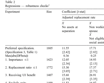
In column 2 of Table 2 we present the results for the specification outlined in 13
the previous paragraph. The important thing to note about this specification is that the coefficient on the adjusted replacement rate (the ‘mean’ effect) is insignificant (and of the ‘wrong’ sign); consequently we exclude this variable and report our preferred specification in column 3. As can be seen, the estimated benefit effects are statistically significant and considerably larger than any others we found. The largest predicted benefit effect is thus for households in the 14 intersection of these two groups — which comprises just over 9% of our sample. Once again we consider the case where the respondent is the sole bread-winner (‘importance’51) and a cut in the replacement rate from 60% to 50% (which constitutes a cut of 17% in the actual benefit paid). The predicted fall in total expenditures is 2.9%, with an associated elasticity of 0.17. Evaluated at the means (for households in the intersection of these two groups), this would be a monthly cut in benefits of about $180 and in total expenditures of about $45 (that is expenditures fall $0.25 for every dollar cut in benefits). Even for these households,
12
There is also an asset disqualification rule in most provinces. We have not built this into our eligibility variable.
13
Only the coefficients on the benefit variables are reported in Table 2; the rest of the coefficient estimates for this specification are presented in the last column of Table 3.
14
Table 2
a Regressions — robustness checks
Experiment Size Coefficient [t-stat] Adjusted replacement rate
X X
No assets at Non working separation spouse
X
Not eligible for social assistance Preferred specification. 1805 11.55 17.71
(Specification 3, Table 1) [2.42] [2.82]
Max(abs(DFbeta)) 0.36 0.25
1. Importance #1 1423 12.05 14.93
[2.36] [2.13]
2. Replacement ratio#1 1772 15.30 17.37
[3.05] [2.71]
3. Receiving UI benefit 1407 15.68 26.91
[2.39] [3.35]
4. Exclude quits 1490 11.53 16.97
[2.21] [2.50]
5. Median regression 1805 6.52 0.84
(Median5 23.1%) [1.16] [0.095]
6. 25% regression 1805 14.34 29.78
(First quartile5 225%) [2.00] [2.05]
7. 10% regression 1805 33.24 46.48
(First decile5 250%) [2.38] [2.79]
a
Alternate estimates of the preferred specification (specification 3 in Table 1). Rows 1 through 4 differ in the estimating sample. Rows 5 through 7 report quantile, rather than least squares regressions. Because of the well-known problems with asymptotic standard errors for quantile regression we report bootstrap standard errors based on 100 replications.
our estimates do not imply equal dollar-for-dollar cuts in expenditures with cuts to benefits.
the coefficient value. The second row of Table 2 indicates that the largest (in absolute value) DFBETA statistics for the coefficients on the replacement ratio variables is less than 0.4. Thus we conclude that our results are not being driven
15 by a small number of outliers.
We turn now to a number of restrictions on the estimating sample. The first experiment concentrates on the ‘importance’ variable. It is motivated by the fact that for many of the respondents the ‘importance’ variable is greater than unity. Unless the household had negative net income for other sources of income than the respondent’s earnings (which is possible) then this must be because of the measurement error in the lagged net income and earnings variables that are used to construct the importance measure. We drop respondents who had ‘importance’ greater than unity; as can be seen the parameter estimates are virtually unchanged. The next two experiments address concerns about the variation in the replace-ment ratio. As can be seen from the statistics presented at the end of Section 3, we have some respondents with a replacement ratio above the statutory rate of around 60% and also a number who do not receive benefit. As explained above, the former is partly the result of the differential tax treatment of benefits and earnings, but in the case of very high replacement rates it is likely a consequence of our measure of past earnings being different from ‘insurable earnings’ and measured with error. To check whether this is biasing our results, we simply exclude those with a replacement ratio of above unity. As the third row of the table reports, the results actually become slightly stronger.
The other concern about the replacement rate is that our results might be driven solely by the variation between those who have no benefit and those who do. In experiment 4 we present the parameter estimates for the sub-sample who have positive benefit (using the ‘preferred’ replacement rate). Here, we find that our results become stronger again. The ‘zero benefit’ group in our sample comprises both individuals who have exhausted their benefits and those who do not take up benefits, including the ineligible. However, conditional on our rich controls we find no difference between these groups.
Next we consider quits. The disentitlement of quitters in 1993 provides an additional source of variation in benefits but to the extent that quits are more voluntary than other job separations one might be concerned that their presence in the sample is endogenously determined by their entitlement. However, as row 5 (experiment 4) of Table 2 illustrates, excluding quits from our sample has a negligible impact on the results.
15
The next set of robustness checks are somewhat different. It is plausible that those who are most sensitive to benefit variations are those who experience the largest fall in expenditure. To check this, we ran three quantile regressions — for the median, first quartile and first decile, respectively. As can be seen from Table 2, expenditure for the three percentiles fall by 3.1%, 25% and 50%, respectively. The parameter estimates given speak for themselves. The effect of the benefit variables is insignificant for the median group whereas it is much larger for those who experience a large fall. Indeed, taking the parameter estimate for the first decile, (and again, assuming ‘importance’ equal to one and focusing on the households in the intersection of our two ‘sensitive’ groups) a reduction in the replacement rate from 60% to 50% would increase the expenditure fall by almost eight percentage points. Our interpretation of these quantile regression results is that some agents are liquidity constrained; they have large falls in expenditure and show a large sensitivity to benefit changes whereas most other agents are not affected by marginal changes in the benefit level and have smaller falls in
16 expenditure.
The bottom line for these robustness checks is that the basic result (see specification 3 in Table 1) seems to be robust to many changes in the empirical specification. Our results are not being driven by a small number of outliers and they seem to be robust to changes in the specification of the importance variable and the replacement rate. On the other hand, there is considerable evidence that the mean effect given seems to be the result of a large effect for a few people rather than a smaller effect for everyone.
5. Discussion
In this paper we have used a survey of workers who separated from a job in early 1993 or 1995 to investigate the ‘consumption smoothing’ benefit of UI. This is not the only benefit from UI but we focus on it because it is often cited as being the most important benefit of UI programs. The consumption smoothing benefit accrues to liquidity constrained households who cannot consume in a manner consistent with their expected future income (making due allowance for prudence). The question of whether households are liquidity constrained has been the central focus of a great number of studies over the past 15 years, but this debate has been
17
remarkably inconclusive. Nevertheless, if any segment of the population is likely to be liquidity constrained it is the unemployed. This is because current income is more likely to be below ‘permanent’ income for this group, they have relatively little in the way of assets and anecdotal evidence suggests that the first thing that many potential lenders consider is the labour force status of the applicant. Thus,
16
Note however, that the theory outlined in Section 2 applies to the means. 17
the role of UI benefits in consumption smoothing remains an important empirical question.
Another reason for focusing on liquidity constraints and the ‘consumption smoothing’ benefits of UI is that a large component of the effect of UI benefits on job search, unemployment spell duration and the quality of a new job may run through this channel. In the standard model of the duration effects of UI benefit, agents have a linear utility function and are indifferent about the timing of consumption. Consequently they simply maximize the present value of income. The presence of a UI benefit distorts search behaviour and causes agents to search ‘too much’. In a search model with strictly convex preferences (and hence a preference for ‘smooth’ consumption) these ‘lifetime budget constraint’ considera-tions would continue to operate but we conjecture that such effects may be small relative to consumption timing effects among the liquidity constrained. The consumption smoothing effect will be to induce constrained agents to stop search (and take a job) ‘too early’. We emphasize that this is conjectural; although the results in Flemming (1978), Danforth (1979) and Ioannides (1981) are suggestive, a full characterization of this problem is the subject of ongoing research.
More generally, we can trace the impact of UI benefits on household behaviour and welfare through the chain: UI benefits→personal income→household income→household expenditures→current household living standards→long run outcomes. In this paper (and in Gruber (1997)) the focus is on the overall link from benefits to expenditures. The link between this and living standards (the purchases of non-durables and services and the service flow from durables and housing) is a complicated one. For example, the mean 14% fall in expenditures seen in our sample could all be for durables, clothing and costs of working. If small durables and clothing depreciate only slowly, then households will maintain living standards (or ‘smooth consumption’) even over a relatively long unemploy-ment spell. In a companion paper (Browning and Crossley, 1999) we develop the idea that agents have access to ‘internal capital markets’ by postponing the purchase of durables during an unemployment spell. Although there is a welfare
18
cost from not replacing a (functioning) durable at the optimal time, this is of second order importance. For example, the service flow from an old undamaged winter coat is almost as great as that from a new one. If this is the case, then large changes in durable expenditures may not be reflected in large changes in service flows and hence welfare. Because most small durables are luxuries, this ‘internal capital markets’ hypothesis has qualitative predictions that are similar to the standard Marshallian predictions but the rationale of the two hypotheses are quite different.
Our findings suggest a very modest and only marginally significant mean impact of benefit levels on household expenditures. Our specific estimate suggests that a
18
10 percentage point cut in the benefit would result in an average fall of less than 1% in total expenditure. In work similar to that reported here, Gruber (1997) uses the PSID to examine the impact of UI benefits on changes in expenditures on food at home and food outside the home. Gruber’s estimates imply that a 10% point cut in the UI replacement rate would lead to an average fall of about 2.5% in food expenditures. The interpretation of Gruber’s results — and the comparison of those with the results reported here — depends heavily on the relationship between changes in food expenditure and changes in total expenditure during an unemploy-ment spell. Gruber states that the response of food and total expenditure should be the same but it is difficult to see why. In a standard Marshallian model, the income elasticities for food at home and food outside are about 0.4 and 1.2, respectively. Given a budget share for food at home that is about three times the budget share for food outside, we have an elasticity of about 0.6 for the composite food commodity. Thus the Gruber results suggest a change of 4% (52.5% / 0.6) for
19 total expenditure which is a good deal higher than our mean effect.
As discussed in Browning and Crossley (1999), there is reason to believe, however, that standard Marshallian demand analysis may not be appropriate for the unemployed. The ‘internal capital markets’ hypothesis suggests that the responses of expenditure on durables to an income loss because of unemployment will be larger than implied by income elasticities estimated on samples of households experiencing ‘normal times’. In Browning and Crossley (1999) we present strong evidence for this contention. This further suggests that changes in food expenditure may be an even smaller fraction of changes in total expenditure than typical food-income elasticities would suggest. Thus all these considerations would suggest that Gruber’s implied estimate of the mean benefit effect for total expenditure is a good deal higher than ours.
Our analysis of the mean effect differs from Gruber’s study in several respects. The most obvious of these is that Gruber uses US data and we use Canadian data. One immediate corollary of this is that we are generally dealing with UI benefit replacement rates that are higher than those for the US. The timing is also different; Gruber uses year-to-year variations in employment status and does not control for how long the unemployment spell is whereas most of our sample have had a spell of between 4 and 9 months. We also employ a different source of variation in UI benefits to identify the transitory response. Gruber uses state level provisions which vary over both time and across states. In Canada, UI benefits are set nationally, and vary only through time. However, our data capture two major sets of legislative changes to the Canadian UI system, as well as some administrative changes. While not as extensive as the variation captured by Gruber’s data, the variation in the Canadian program parameters is substantial and transparent. One concern with Gruber’s approach is that it identifies the
(tempor-19
ary) ‘benefit’ effect only if state level variables are uncorrelated with permanent shocks from a job separation. For example, if states have to balance their UI accounts then benefit levels will be lower the worse is the unemployment situation. If the latter is also correlated with a larger negative shock from a job loss then part of the effect in Gruber’s base estimates could be due to the negative correlation between benefit levels and the permanent shock. If in a regression of expenditure changes on benefit levels there is a positive coefficient on the latter then this may be partly due to the direct benefit effect (due to liquidity constraints) and partly due to the negative correlation between job separation shocks and expenditure changes. However, Gruber’s results seem robust to attempts to deal with this issue, including conditioning on state fixed effects.
It is also possible that the differences in our results arise because of differences in the population of unemployed between Canada and the US, or in differences in the smoothing mechanisms available to the unemployed in the two countries. Given the expenditures on unemployment insurance in western economies, and the relative lack of empirical research on the benefits of unemployment insurance, estimates on various samples and using alternative sources of variation in benefit levels would seem important.
Although we find only a small mean effect, our most important finding is that the benefit effect is very heterogeneous. Most unemployed households seem to be insensitive to marginal changes in the level of benefit. The results presented in Table 1 (and the specification checks presented in Section 4) suggest that there are substantial effects for some households that did not have liquid assets at the job separation and / or in which there is a spouse who is not employed. The quantile regressions presented in Table 2 point even more clearly toward the conclusion that benefit effects are concentrated on a small proportion of our sample (about 10%) but for them there is close to a one–one relationship between UI benefit levels and total expenditure (as theoretical models of liquidity constraints would suggest). Moreover, these same households are the ones which have had to cut expenditure the most. This finding of considerable heterogeneity suggests that conclusions drawn from studies that use a representative agent framework (such as Bailey (1978)) may be misleading.
UI benefits. These households are those that had little in the way of assets or access to credit and which experienced a large fall in total expenditure. Although the implications for policy from this finding have yet to be fully analysed it is clear that the consumption smoothing gain from UI (which many believe to be the most important gain) will depend heavily on the weight given to the small group who have substantial welfare gains from increases in UI benefits.
Table A.1
a Controls — means, notes and coefficients from preferred specification
Variable Mean Notes Coeff. [t-stat]
Constant 23.940 [20.9]
Importance 0.50 Lost earnings / household income 210.450 [23.06] Highschool 0.39 Dummies; less than highschool 20.020 [20.02] College 0.28 is the omitted category 20.320 [20.2]
Age 20.23 Decades from 40 2.170 [3.31]
Ln(household size) 0.94 21.380 [20.73]
Male 0.48 Dummy 20.010 [20.01]
Married, spouse not empl. 0.23 Dummies; married, spouse 1.610 [0.8] Single 0.18 employed at job loss is the 23.340 [21.14] Other household 0.10 omitted category 24.090 [21.9]
Atlantic 0.12 Dummies; Ontario is the 7.290 [3.36]
Quebec 0.30 omitted category 0.860 [0.56]
Prairies 0.14 2.280 [1.24]
BC 0.10 20.610 [20.3]
Assets at job loss 0.33 Dummy; investment income in 23.340 [21.68] previous tax year
Home owner 0.58 Dummy 3.210 [2.35]
% of household income 0.30 (mortgage payment or rent) / 8.730 [3.39] committed household income at interview
Eligible for social 0.26 Dummy 21.690 [20.9]
assistance
Expected job loss 0.56 Dummy 1.240 [1.01]
Seasonal job 0.16 Dummy 1.290 [0.74]
Long tenure job 0.56 Dummy 0.020 [0.01]
Manager 0.25 Dummy; white collar, non-manager 22.200 [21.45] Blue collar 0.33 is the omitted category 1.340 [0.87] UI use in 1 of 2 previous years 0.59 Dummy 1.530 [1.17]
Weeks work in year before 30.6 20.090 [22.1]
job loss
Local unemployment rate 0.11 16.620 [0.99]
Ln(earnings last year) 1.05 $1000s / month 20.040 [20.03] Ln(earnings 2 years previous) 0.97 22.490 [21.84] Ln(earnings on lost job) 0.43 $1000 / month 0.770 [0.34]
squared 20.120 [20.1]
cubed 20.500 [20.64]
a
Acknowledgements
We are grateful to Roger Gordon, two anonymous referees and participants in the TAPES Conference, Copenhagen, 1998 for their comments as well as to Thierry Magnac and participants at several seminars for comments on an earlier version of this paper (Browning and Crossley, 1996) employing only the 1993 COEP. We acknowledge financial support from the Social Science and Humanities Research Council of Canada. The data used in this study were made available by Human Resources Development Canada. The latter bears no responsibility for the analysis nor for the interpretation of the data given here.
Appendix A
Table A.1 provides additional information on our controls for the permanent shock of job loss, demographics and other determinants of expenditure. Column 1 lists these variables. Column 2 gives their mean in our sample, and column 3 provides some further information. The final column presents the estimate coefficient (and related t-statistic) for each variable in our preferred specification (the coefficients on benefit variables in this specification were presented in column 3 of Table 1).
References
Angrist, J., Krueger, A., 1998. Empirical Strategies in Labor Economics. Handbook of Labor Economics, In press.
Bailey, M., 1978. Some aspects of optimal unemployment insurance. Journal of Public Economics 10 (3), 379–402.
Browning, M., Crossley, T., 1996. Unemployment insurance benefit levels and consumption changes, Department of Economics, McMaster University, Working paper 96-04.
Browning, M., Crossley, T., 1999. Shocks, stocks and socks: consumption smoothing and the replacement of durables during an unemployment spell, Australian National University, Working paper in Economics and Econometrics no. 376.
Browning, M., Lusardi, A., 1996. Household saving: micro theories and micro facts. Journal of Economic Literature 34, 1797–1855.
Chamberlain, G., 1984. Panel data. In: Griliches, Z., Intriligator, M.D. (Eds.), Handbook of Econometrics, Elsevier, Amsterdam, pp. 1247–1313.
Chaterjee, S., Hadi, A., 1988. Sensitivity Analysis in Linear Regression, Wiley, New York. Danforth, J., 1979. On the role of consumption and decreasing absolute risk aversion in the theory of
job search. In: Lippman, S., McCall, J. (Eds.), Studies in the Economics of Search, North Holland, New York.
Gruber, J., 1997. The consumption smoothing benefit of unemployment insurance. American Economic Review 87 (1), 192–205.
Hamermesh, D., 1982. Social insurance and consumption. American Economic Review 72, 102–113. Ioannides, Y., 1981. Job search, unemployment and savings. Journal of Monetary Economics 7,
355–370.