Addressing uncertainty in medical
cost–effectiveness analysis
Implications of expected utility maximization for
methods to perform sensitivity analysis and
the use of cost–effectiveness analysis to
set priorities for medical research
David Meltzer
∗Section of General Internal Medicine, Harris Graduate School of Public Policy Studies, Department of Economics, University of Chicago, 5841 S. Maryland Avenue MC 2007, Chicago, IL 60637, USA
Received 1 April 1999; accepted 29 August 2000
Abstract
This paper examines the objectives for performing sensitivity analysis in medical cost– effectiveness analysis and the implications of expected utility maximization for methods to per-form such analyses. The analysis suggests specific approaches for optimal decision making under uncertainty and specifying such decisions for subgroups based on the ratio of expected costs to expected benefits, and for valuing research using value of information calculations. Though ideal value of information calculations may be difficult, certain approaches with less stringent data re-quirements may bound the value of information. These approaches suggest methods by which the vast cost–effectiveness literature may help inform priorities for medical research. © 2001 Elsevier Science B.V. All rights reserved.
JEL classification: I18; D61; O32
Keywords: Cost–effectiveness analysis; Uncertainty; Sensitivity analysis; Health care research; Value of information; Welfare economics
∗Tel.:+1-773-702-0836; fax:+1-773-834-2238.
E-mail address: [email protected] (D. Meltzer).
1. Introduction
Despite some recent slowing in the growth of health care costs in the US, health care costs have risen substantially over the past several decades and are likely to continue rising (Smith et al., 1998). This appears to be largely due to the growth of new technology (Fuchs, 1990; Newhouse, 1992). While improvements in health are highly valued (Cutler and Richardson, 1997; Murphy and Topel, 1998), evidence from diverse methodological perspectives sug-gests that many technologies may have little value at the margin (Eddy, 1990; Brook et al., 1983; McClellan et al., 1994). Cost–effectiveness analysis and other methods for medical technology assessment have arisen to attempt to address this important problem.
One of the main challenges faced by medical cost–effectiveness analysis has been the question of how to perform these analyses in the presence of uncertainty about the benefits and costs of medical interventions. The uncertainty of primary interest in this regard is uncertainty in population level outcomes, although uncertainty in outcomes at the individual level may be present simultaneously. This uncertainty in population level outcomes may result either from limited evidence from clinical trials or the need to extrapolate based on the results of clinical trials using decision analysis and its associated uncertainties in the structure and parameters of decision models. This uncertainty concerning the benefits and costs of medical interventions has motivated much interest in sensitivity analysis within medical cost–effectiveness analysis.
Yet though there have been many proposals about how to address uncertainty in cost– effectiveness analysis, there has been relatively little discussion of the objectives for per-forming sensitivity analysis. Without a clear understanding of these objectives, it is difficult to know by what criterion to assess the merits of the many alternative approaches to sen-sitivity analysis. Thus, the lack of clarity concerning the objectives for sensen-sitivity analysis is an important reason for the continuing ambiguity about how to address uncertainty in cost–effectiveness analysis.
costs to expected benefits for that subgroup is the appropriate criterion. If the objective of sensitivity analysis is to set priorities for the acquisition of additional information, then the incremental increase in expected utility with additional information is the appropriate measure of benefit. Though such ideal value of information calculations may be difficult to perform, other approaches to sensitivity analysis with less stringent data requirements may provide bounds on the value of information. Together, these approaches suggest a theoretically grounded approach by which the tools of medical cost–effectiveness analysis can be used to help set priorities for medical research. Following these approaches, it may be possible to draw upon the vast literature on the cost–effectiveness of specific medical interventions (Elixhauser et al., 1998) to address crucial needs for more systematic ways to set priorities for medical research. After active discussion between Congress, the Ad-ministration, and the leadership of the National Institutes of Health (NIH) over the value of and priorities for Federal funding of biomedical research, the need for such systematic approaches to identify priorities for research at the NIH was recently highlighted in a report of the Institute of Medicine (IOM, 1998).
Section 2 discusses the objectives of sensitivity analysis. Section 3 discusses the primary methods currently used to perform sensitivity analysis. Section 4 uses an expected utility maximization model to derive methods for optimal decision making in the context of un-certainty about population outcomes. Section 5 extends the basic results of Section 4 to encompass uncertainty at the individual level. Section 6 uses the model to derive methods for sensitivity analysis to guide decisions for individuals or subgroups that differ from a base case. Section 7 applies these principles to a stylized decision concerning a medical treatment of uncertain benefit. Section 8 uses the model to derive methods to use sensitivity analyses to inform priorities for the collection of additional information to guide decision making, including approaches to bound value of information calculations with limited information. Section 9 applies these ideas to a stylized model of the decision whether to treat prostate cancer and discusses some challenges in implementing these approaches to set priorities for research. Section 10 concludes.
2. Objectives for sensitivity analysis
In order to begin to assess methods to account for uncertainty in cost–effectiveness analy-sis, it is essential to consider the objectives in performing sensitivity analyses. Although not all of these objectives may be relevant in every application, the objectives appear to fall into three broad categories: (1) to help a decision maker make the best decision in the presence of uncertainty about costs and effectiveness, (2) to identify the sources of uncertainty to guide decisions for individuals or groups with characteristics that differ from a base case, and (3) to set priorities for the collection of additional information.
2.1. Decision making under uncertainty about cost and effectiveness
confidence. Nevertheless, patients must decide whether they want the immunization and public and private insurers must decide whether they will cover it. Thus, having a mechanism to help guide decision making when the costs and benefits of a medical intervention are uncertain is important.
2.2. Decision making for individuals or subgroups that differ from a base case
Though not frequently stated as a motivation for sensitivity analysis, developing insight into decisions faced by individuals or subgroups is also a common motivation for performing sensitivity analysis in medical cost–effectiveness analysis. For example, a cost–effectiveness analysis for immunization of a population would likely consider the average risk of ac-quiring an infection in the absence of immunization. However, an analyst examining the cost–effectiveness of immunization for an individual or group with a known risk factor for acquiring some infection would want to reflect that higher-than-average risk.
2.3. Priority-setting for the collection of additional information
When the conclusions of a cost–effectiveness analysis are altered by parameter values that cannot be ruled out based on the literature, the collection of additional information concerning those parameters may be justified. Though in practice it is not frequently done, sensitivity analysis can be used to identify parameters that may change the results of a decision analysis and those parameters may then be studied more intensively. A few studies have used this approach to determine the value of sample size for clinical trials (Claxton and Posnett, 1996; Hornberger, 1998), or to perform sensitivity analysis in a decision model by calculating the expected value of perfect information concerning specific parameters of the model (Felli and Hazen, 1998).
Although these three motivations for performing sensitivity analysis are clearly distinct, papers in the literature commonly do not distinguish among them in their discussion of the sensitivity analysis. This is important because different methods for sensitivity analysis may be better suited to different objectives. This is discussed further below.
3. Methods for sensitivity analysis
Before attempting to derive methods for performing sensitivity analysis, it is useful to discuss the existing methods. The oldest and most commonly used forms of sensitivity analysis are univariate sensitivity analyses. Following these approaches, analysts begin with the mean or modal values of all the probabilities in their analysis and use those to calculate the costs and benefits for a “base case” analysis. The parameters are then varied individually across a range of possible outcomes to see how the cost–effectiveness of an intervention changes. In some instances, the parameter values are varied over the range of all possible values, while in other cases they are varied across confidence intervals that are drawn from the medical literature.
are also a number of significant shortcomings of these approaches. First, they do not clearly delineate either what range of parameter values to consider or what to do when some of those possible parameter values would change the optimal decision. For example, consider again the case of a vaccination. Its probability of providing immunity is logically constrained to a number between 0 and 1. High and low estimates in the literature might be 0.98 and 0.60. The best study might predict a protection rate of 0.92 with a 95% confidence interval of 0.89–0.96. Which of these are we to choose in setting the range of parameters? If we choose the broadest range, it may be impossible to pin down the costs and benefits with sufficient precision to determine whether the intervention is worthwhile. If we use a 95% confidence interval and find a benefit throughout the range, the potential for an immense harm that could occur if the true value of the parameter falls outside that range would fail to be recognized. Even if we find that the optimal decision changes for a parameter value at the upper end of the 95% confidence interval, it is not clear how that should change the decision we should make. If the welfare benefits over the majority of the interval are large, and any welfare loss at an extreme of the confidence interval is modest, it is not clear that the negative result at the extreme should have much influence on the decision made. Threshold analyses — which identify the parameter values at which an analysis crosses a cost–effectiveness threshold — are subject to the same criticism for failing to reflect the magnitude of the effect of the parameter on costs and outcomes and therefore the significance of the fact that the cost–effectiveness ratio crosses some threshold for some parameter values.
Another concern with one-way sensitivity analyses is that they may be misleading if the results obtained by varying a parameter depend on the level of other parameters in the model. This has motivated multi-way sensitivity analyses in which parameters are varied simultaneously across plausible or likely ranges. These analyses are subject to all the con-cerns described above concerning one-way sensitivity analyses, as well as some additional problems. One problem with these approaches is that the number of sensitivity analyses that must be performed rises exponentially with the number of parameters. Another prob-lem is that assumptions about one parameter often have implications for assumptions about other parameters. For example, assumptions about the natural history of untreated disease may have implications for the history of disease under treatment. This has motivated ef-forts to examine the joint distribution of the parameters in a model. This approach, along with a similar population-based sampling approach to estimating costs, effectiveness and cost–effectiveness ratios, sometimes termed stochastic cost–effectiveness analysis, appears to be receiving increasing attention in the field (O’Brien et al., 1994; Gold et al., 1996; Polsky et al., 1997). However, these analyses still do not address the question of the optimal decision in the presence of uncertainty because they do not suggest what to do when the set of possible costs and outcomes include ones that would make the cost–effectiveness ratio fail to meet the chosen threshold for cost–effectiveness.
cost–effectiveness ratios would not generally be meaningful (Stinnett and Paltiel, 1997). One creative approach to these issues is to reformulate cost–effectiveness analyses in terms of Net Health Benefits (Stinnett and Mullahy, 1998), in which both costs and benefits are expressed in the common denominator of years of life saved. While free of some of the complications associated with estimating cost–effectiveness ratios, the utility of the Net Health Benefit approach is diminished by the fact it does not allow easy comparisons with results from traditional cost–effectiveness analyses that rely on cost–effectiveness ratios, and is dependent on assumptions about the valuation of improvements in health. A related approach with similar concerns is to convert health benefits into a monetary value, as is done in cost–benefit analysis (Tambour et al., 1998).
In assessing these methods, it is interesting to note that while all of them appear to have some significance for the objectives described above, none of them are explicitly linked to those objectives. As discussed above, this lack of clarity concerning the objectives for sensitivity analysis is an important reason for the continuing ambiguity concerning methods to account for uncertainty in medical cost–effectiveness analysis. The next two sections use an expected utility maximization model to attempt to develop an approach to assess the importance of uncertainty about parameter values in order to make an optimal decision under uncertainty. The sections that follow then examine the adaptation of that approach to address the other two common objectives of sensitivity analysis — the determination of cost–effectiveness for individuals or subgroups and the identification of areas where the collection of additional information would be of value.
4. A deterministic model of health outcomes with uncertainty about effectiveness
In this simple case, we assume that there is uncertainty about the effectiveness (θ∈Θ, with pdf p(θ)) of providing m units of medical care (for example, blood pressure checks per year), but that the outcome of that medical care givenθ is certain. By making this assumption, we abstract from the problem of uncertainty in outcome for an individual, and focus instead on uncertainty for a “representative consumer” assumed to be identical to all other individuals, so that there is no heterogeneity in the population. We return to these issues of individual level uncertainty and heterogeneity in Sections 5 and 6, however.
To capture the possibility that effectiveness may affect both the costs and benefits of an intervention, we allow both utility (U) and the costs of the medical care (c) to depend directly onθsoc=c(m, θ ). This allows the cost of m units of medical care to be uncertain, as it might be, for example, if it is not known how much those blood pressure checks and resulting treatments would cost. In addition, utility is assumed to depend on non-medical consumption (x) and medical expenditure, so U = U (m, θ, x(θ )). Here x is written as x(θ) to denote the fact that x will vary withθ for any m to satisfy the budget constraint
c(m, θ )+x(θ )−I =0 for each level of effectiveness. To model cost–effectiveness, we
assume that people maximize expected utility1 and take the example of a representative
1While individual preferences may in fact be inconsistent with expected utility maximization, QALYs implicitly
consumer who maximizes expected utility subject to budget constraint conditional on each
Rewriting this as a Lagrange multiplier problem withλ(θ) as the multiplier for the budget constraint at each level ofθ, and multiplying eachλ(θ) by p(θ) without loss of generality yields
This generates a first-order condition for medical expenditure which is
Z
This implies that investment in a medical intervention should occur to the point at which its expected marginal benefit (utility) equals the expected value of the marginal-utility-of-income-weighted marginal cost. Allowing the marginal utility of income to depend onθ
reflects the possibility that, either because of changes in the utility function or costs withθ, income might have a greater or lesser marginal utility.
For an individual, these effects of uncertainty about the costs and effectiveness of medi-cal interventions on the marginal utility of income are clearly plausible and potentially important. If someone has hip replacement for arthritis at age 55 and then suffers a severe complication, is forced into early retirement, and requires around-the-clock care, both their utility and medical costs will be directly affected and their marginal utility of income could change substantially. In a population, however, such effects are far less compelling because insurance can equate the marginal utility of income across health states unless an interven-tion leads to an extraordinarily large change in either populainterven-tion health or costs. Thinking from a population perspective in which most extremely expensive medical interventions affect a relatively small number of persons and most common medical interventions are rel-atively modest in cost, it is much less likely that the (aggregate) marginal utility of income will change substantially with uncertainty about the costs or benefits of a single interven-tion.2 If this is the case, then limλ(θ ) → λ and the first-order condition for medical expenditures converges to
which implies that the cost–effectiveness ratio is
R
2Note that even if changes in health status led to substantial changes in income or the need for non-medical
Thus, expected utility maximization implies that the optimum cost–effectiveness ratio of an intervention in a population under uncertainty is closely approximated by the ratio of expected costs to expected benefits. Note that this “ratio of means” solution is analogous to that suggested by Stinnett and Paltiel (1997) as the solution to a constrained optimization problem in a linear programming context and by Claxton (1999) in a Bayesian discrete choice decision theoretic context. However, neither analysis derives the result directly from a formal utility maximization model nor addresses the possible dependency of the marginal utility of income onθ.
While this argument about the dependence of the marginal utility of income onθhas not been made previously in the context of medical cost–effectiveness analysis, it should be noted that the argument is quite similar to that made by Arrow and Lind (1970) concerning the evaluation of risk in public investment decisions. There the authors argue that the large scale of the public sector allows it to effectively eliminate any welfare loss associated with the riskiness of investments by spreading the risk across a sufficiently large population. The argument here relies both on this diversification effect and the relatively modest magnitude of almost any one public health care decision in the context of overall health and health expenditures.
5. A stochastic population model with individual-level uncertainty about outcomes
Unlike in the deterministic model presented above, medical interventions almost always have uncertain outcomes for individuals even when there is no population-level heterogene-ity so that all individuals share a common set of parameters (θ). Thus, for a set of individuals indexed byj ∈ J who might each experience health outcomeεj ∈E, the probability of
experiencing outcomeεjgivenθ∈Θcan be written as f(εj|θ) and expected utility can be
written as
Z
p(θ )
ZZ
f (εj|θ )Uj(m, εj, xj(εj, θ ))dεjdjdθ such that
cj(m, εj, θ )+xj(εj, θ )−I =0 for all θ, j, εj. (6)
Following the lines of the argument above, we can construct state-specific Lagrange mul-tipliersλj(εj, θ )and note that if there is (1) a large population so that aggregate risk given
θis negligible, (2) full insurance, and (3) uncertainty in the effectiveness of the interven-tion has limited consequences in the sense thatθdoes not have much effect onλas described above, then
limλj(ε, θ )E →λ(Eε, θ )→λ for all Eε≡ {ε1, . . . , εj, . . . , εJ},where
εj ∈E and for all θ. (7)
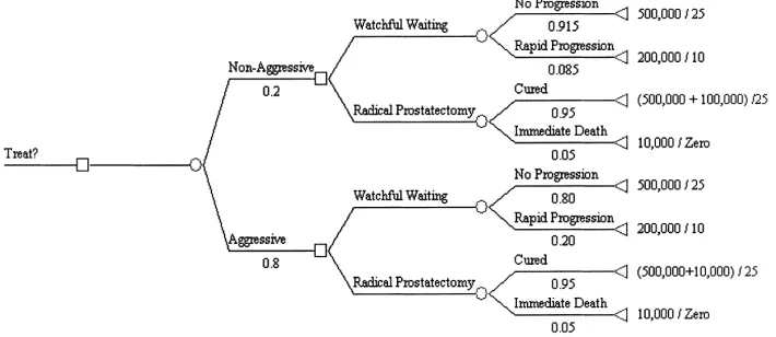
Fig. 1. Simplified decision concerning a treatment of uncertain benefit (cost (US$)/effectiveness (life years)).
6. Sensitivity analysis to guide individual or subgroup decisions
When sensitivity analysis is done to guide decisions for individuals or subgroups, the problem is essentially the same as for the total population, except that the parameter vector
θ has a different probability distribution p′(θ) than in the overall population. This may occur if parameters for those individuals or subgroups are thought to differ from those for the population as a whole. This is the type of heterogeneity that most frequently motivates subgroup analyses in cost–effectiveness analysis. However, subgroup analysis may also be desirable if the values of the parameters for a subgroup are not known to differ from those in the population as a whole, but the subpopulation is more or less well studied. In both cases, the analysis differs only in the probability distribution for the parameters, with cases in which some parameters for subgroups are known with certainty addressed by a simplification of the analysis in which the marginal density for the known parameters is degenerate because there is no uncertainty about them.3 Accordingly, the solution to this problem for individuals or subgroups is again the ratio of the expected value of costs to the expected value of benefits, only using the appropriate prior probability distribution for the subgroup or individual.
7. Application to a stylized decision concerning a treatment of uncertain benefit
Fig. 1 describes a stylized decision concerning an intervention of uncertain benefit. For simplicity, the intervention is assumed to cost US$ 10,000 with certainty. Uncertainty is assumed to exist only with respect to benefits; it is assumed that there is a 90% chance
3To illustrate: let Groups A and B have pdfs pA(θ) and pB(θ). Now assume that this heterogeneity can be fully
parameterized and partitioned into a certain part (θC) and an uncertain part (θU) so that these pdfs can be fully
parameterized aspA(θ )=p(θA
U;θCA) andpB(θ )=p(θUB;θCB). In this case, the differences in the certain parameters
(θC), can be viewed as representing observable heterogeneity, while the uncertainty over the uncertain parameters described by the pdfs describes the uncertainty with respect to which decisions need be made (i.e. integrated over
that the benefit is 0.1 life year, but also a 5% chance each that the benefit is 0.01 or 1 life year.
Taking these three possibilities individually, the cost–effectiveness ratios are US$ 100,000, 1,000,000, or 10,000, respectively. If one used a cutoff of US$ 100,000 per life year, a tra-ditional sensitivity analysis would therefore be indeterminate. Indeed, such indeterminacy is extremely common in cost–effectiveness analyses. Another limitation of this standard approach is that, while the cost–effectiveness ratios tell us something about the magnitude of benefits relative to costs, they do not provide any indication of how to incorporate the likelihood of those benefits. Common approaches to sensitivity analysis might take other perspectives. For example, the stochastic cost–effectiveness approach might conclude that since there is only a 5% chance that the intervention is not cost-effective, it should be se-lected. On the other hand, the same approach could be used to argue that since there is only a 5% chance that the intervention will provide a benefit in excess of its cost, it should not be selected. The problem with these perspectives is that they do not reflect the magnitude of potential benefits relative to costs.
Following the expected utility approach described above, the expected cost is US$ 10,000 and the expected benefit is: 0.05×0.01+0.9×0.1+0.05×1.0=0.0005+0.09+0.05= 0.1405 life years. Thus, the cost–effectiveness ratio is US$ 10,000 per 0.1405 life years is equivalent to US$ 71,174 per life year saved, which is clearly cost-effective by the US$ 100,000 per life year standard. Even though the chance that the intervention is highly beneficial is only 5%, more than one-third (0.05/0.1405=36%) of the expected benefit comes from the unlikely event that it is highly effective. It is this ability to incorporate both the magnitude and likelihood of benefits and costs into a single statistic that can be used to guide decision making that is the primary advantage of the expected value approach over the traditional approaches that incorporate only one or the other dimension, and often result in indeterminate conclusions that do not provide much guidance for decision making.
8. Sensitivity analysis to guide information collection
Two exceptions to this are Claxton and Posnett (1996) and Hornberger (1998), which focus on the determination of optimal sample size for a clinical trial from a cost–effectiveness perceptive in a full Bayesian context.
Adopting the expected utility approach, assume that for any information set describing the parameter distribution, p(θ), there is an optimal choice of m as described above. Call
thism∗(p(θ )). This implies an expected utility with existing information (EU0) of
Z
p(θ )U (m∗(p(θ )), θ, x(θ ))dθ. (8)
Now imagine that we are able to acquire additional information aboutθ. Assume further that the cost of this research is cr. Though the analysis is easily generalized to permit an
infinite number of possible outcomes of the experiment,4 assume for simplicity that there are only two possible outcomes of this experiment: with probability q that the distribution ofθis found to be p′(θ) and with probability (1−q) that it is found to be p′′(θ), where, for
with the collection of information, or expected value of information (EVI) is
q
Z
p′(θ )U (m∗(p′(θ )), θ, x∗′(θ ))dθ+(1−q)
Z
p′′(θ )U (m∗(p′′(θ )), θ, x∗′′(θ ))dθ−EU0. (10)
4In the general case, we wish to compare the expected utility resulting from the optimal decision m∗given the
original budget constraint in the absence of information to the expected utility resulting from the optimal decision in the presence of the new information subject to a budget constraint that includes the cost of collecting information (cr). Thus, we compare the expected utility resulting from the solution to
max
Table 1
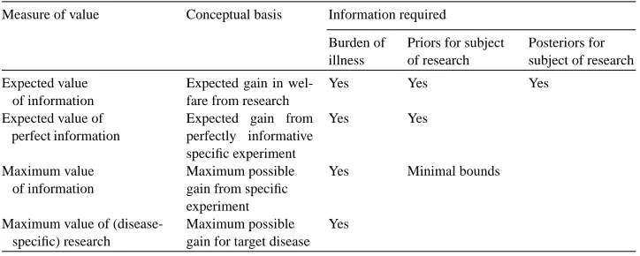
Information requirements for value of information calculations
Measure of value Conceptual basis Information required Burden of
If this is positive then the study is worth performing, if not, then it should not be performed.
Although this value of information calculation is easily described in theoretical terms, implementing this approach requires meaningful information on the prior probabilities of the parameters required for the calculation, and this may be very difficult to obtain. In some instances, priors may be estimated based on published estimates of means and confidence intervals or other data from the literature. In other instances, primary data collection may be required. Still, it is likely that in a significant number of cases it will not be possible to identify much information that will inform priors. Moreover, it may be quite difficult to say much about how an experiment is likely to affect the posterior distributions of the parameters.
These empirical challenges suggest that techniques for assessing the value of information that do not rely on this data concerning prior or posterior distributions would be highly use-ful. Table 1 summarizes a number of such approaches and their informational requirements. In the case where information on priors is available, one such possibility is the expected value of perfect information: EVPI = R p(θ )U (m∗(θ ))dθ−EU0, where m∗(θ) is the
optimal choice of m ifθis known. Since the expected value of information is always posi-tive,5 this provides an upper bound on the ideal value of information calculations described above.
5To see this, note that if research cost are zero, the fact that m∗(p′(θ)) and m∗(p′′(θ)) are optima implies that the
first two terms in the equation are greater than
q
From a practical point, however, the advantage of the EVPI calculation is that it does not depend on the posteriors. Indeed, this is probably one reason why the EVPI approach has been used in the cost–effectiveness literature (e.g. Felli and Hazen, 1998).6
Although EVPI is simpler to determine than EVI, it still depends on knowledge of the priors. An alternative measure that did not depend on this might also be useful. One such measure is the maximal value of information (MVI) over all possible values ofθ ∈ Θ,
MVB=maxθ∈ΘU (m∗(θ )). Although this will also only be an upper bound on EVPI and,
therefore, EVI, it depends only on knowing the value function conditional onθ. Although it may be a relatively crude upper bound, it is worth noting that this criterion in fact corresponds to that implied by a threshold analysis in which the bounds are determined by the extreme values of the parameter (assuming, as is usually done, that the value function is monotonic with respect to the parameters). Thus, applying the threshold technique based on the full range of possible values of a parameter can be considered a bound on the more general value of information calculation, only with less rigorous information requirements. Thus, like EVPI, the threshold approach based on the full range of values a parameter might take can be considered a method to place an upper bound on the more complex EVI calculation. When these calculations suggest that the MVI or EVPI is low, the full EVI calculation is not necessary. Note, in contrast, that the common practices of assessing cost–effectiveness at a 95% confidence interval for a parameter or calculating stochastic cost–effectiveness intervals have no clear theoretical justification.
Thinking more broadly, ifΘ is enlarged to include any conceivable value ofθ, even if the value is not possible with current technology, this type of reasoning can be extended to consider any possible research on the parameter in question. For example, if the probability of cure with the best current treatment for a disease is known to be between 20 and 40% with certainty and the treatment is found not to be worthwhile (perhaps because of morbidity), one could calculate whether treatment would be worthwhile if the cure rate were 100%. This might be called the maximum value of research (MVR), and, in turn, can be used to generate an upper bound on MVI that does not require any data at all concerning the parameter in question. The MVR concept could also be expanded to consider innovations that led to fundamental changes in the structure of the decision tree, and not just the effects of changes in its parameters.
6It should be noted, however, that Felli and Hazen (1998) consider the EVPI relative to the expected value of
9. Application to a stylized model of the decision whether to treat prostate cancer
In order to illustrate these approaches, this section examines a simplified model of the decision to treat prostate cancer. A highly stylized model is chosen to focus attention on the methods rather than the specific application. In this simplified model (Fig. 2), the decision to treat prostate cancer is viewed as a choice between radical prostatectomy (surgical removal of the prostate) and “watchful waiting” (no intervention unless the cancer is found to spread). This decision is represented by the two decision nodes in the middle of Fig. 2. In this simplified model, radical prostatectomy is assumed to be curative, so that the patient lives out a “normal” life of 25 years. However, radical prostatectomy is assumed to have a 5% mortality rate. The outcome of watchful waiting depends on how quickly the cancer progresses. Many cancers will progress slowly enough that men die of other causes before they die of prostate cancer and thus live a normal life of 25 years. Other men will progress rapidly and are assumed to die of prostate cancer at 10 years. For simplicity, we assume that quality of life is not a concern so that outcomes are measured in life years, which are the same as quality-adjusted life years. Radical prostatectomy is assumed to cost US$ 10,000 and the basic future costs of survival are assumed to be US$ 20,000 per year. (See Meltzer (1997) for a justification for including costs of this nature.)
However, the natural history of prostate cancer is not as well understood as suggested by these assumptions. In fact there is much uncertainty even about average rates of progression to death from prostate cancer, i.e. how aggressive the disease is on average. This is the dimension of uncertainty on which we focus in this example. This is captured in a stylized way in Fig. 2 by the upper and lower decision trees that differ in the fraction of tumors that are assumed to progress rapidly (0.085 in the “non-aggressive” case, and 0.2 in the “aggressive” case).
Panels 1 and 2 of Table 1 show the results of a cost–effectiveness analysis of the treatment decision in the non-aggressive and aggressive cases. In both cases, treatment provides a benefit, but in the first case it is a small benefit with a cost per QALY of US$ 420,000 and in the second case it is a much larger benefit with a cost per QALY of only US$ 26,000. If we assume for simplicity that the cutoff for cost–effectiveness is US$ 100,000 per QALY, then the optimal decision in the first case would be watchful waiting, while in the second it would be treatment.
The left most part of the decision tree reflects the fact that we do not know which of these possibilities is the case and places some prior probabilities on the two arms (0.2 aggressive, 0.8 non-aggressive). Panel 3 of Table 1 reports the expected benefits and costs of the screening decision with these priors. In that case, the ratio of the expected costs to expected benefits is US$ 47,000, which is cost-effective by the US$ 100,000/QALY standard. This might seem surprising because of the 80% chance that progression was not aggressive, and treatment is not even close to cost-effective by the US$ 100,000/QALY standard in that case. The result is driven by the 20% chance that the benefit could be much larger, even though that possibility is not very likely. This points out the potential for the ratio of the expected value approach to generate different results than the standard probabilistic approaches based on thresholds for defining cost–effectiveness that do not account fully for both the magnitude and likelihood of the potential benefits.
We now turn to the question of whether the collection of additional information would be of value. Following the approach described above, we begin by calculating the maxi-mum value of information. This calculation can be done in several ways requiring pro-gressively more information. To take an extreme example, assume that we knew nothing about the probability that prostate cancer is aggressive, but only the life expectancy of patients with aggressive cancers who are treated or not treated, and the price of prosta-tectomy. In the absence of knowledge about the probability that cancers would progress rapidly, there is no clear guidance about whether watchful waiting or prostatectomy domi-nates, so we consider both cases as reference cases. Assume first that no treatment is the reference point. To get an upper bound on the value of information, one could use only information on the life expectancy of treated and untreated patients and assume that all patients have aggressive cancers. Specifically, assuming that men who have prostate cancer but are not treated live 10 years (QALYs), while men who are treated live 25 years (QALYs), the value of treatment would be 15 QALYs×US$ 100,000/QALY = US$ 1.5 million per patient. Alternatively, we could assume that that treatment is the reference case, so that the benefit of determining that treatment was not cost-effective would be the cost savings from avoiding prostatectomy (US$ 10,000) and avoidance of treatment-related mortality (0.05 mortality×25 QALYs×US$ 100,000/QALY =US$ 125,000) net of any benefits of treatment, which add to no more than US$ 135,000 per patient.
if the baseline strategy is watchful waiting and US$ 0.135 million×100,000/0.03=US$ 450 billion if the baseline strategy is prostatectomy. These extremely large estimates of the maximum value of information suggest the potential for information of immense value to come from knowledge about the efficacy of prostate cancer treatment, and exceed the cost of any conceivable clinical trial.
Of course these MVI calculations are an upper bound, and a fair interpretation of these findings is that the MVI is simply not informative in this case, despite its analytical simplicity and independence of assumptions about the fraction of cancers that are aggressive. This suggests that it is worthwhile to pursue the expected value of perfect information (EVPI) approach.
The EVPI approach is described in panel 4 of the table. The panel describes the expected value of three strategies: watchful waiting, radical prostatectomy, and the optimal decision with perfect knowledge of the average progression rate (EVPI). The last two columns report the value of the change in QALYs (assuming US$ 100,000/QALY for illustration) and the net incremental benefit of the policy choice compared to the strategy immediately above it in Table 2.
The first point to note is that if one made policy based on the most likely cost–effectiveness ratio (US$ 420,000), one would choose watchful waiting, but if one chose based on the ratio of the expected values, one would choose radical prostatectomy, which yields a net benefit of US$ 19,600 (US$ 26,000−6400) per patient relative to watchful waiting. This is a quantified measure of the expected gain from the improvement in decision making by using the mean of the expected values as opposed to basing the decision on the most likely cost–effectiveness ratio, as is generally done in the “base case” reported by most current cost–effectiveness analyses.
The second point to note is that the expected value of the gain versus watchful waiting with improved information is even higher at US$ 26,000 per patient. This implies an additional gain of US$ 6400 per patient of the improved information compared to the best possible decision with the initial information. Converting this patient level estimate of the value of research into a population level estimate as above suggests an EVPI of US$ 6400× 100,000/0.03=US$ 21 billion. As with the MVPI, this large EVPI suggests that the value of information about the efficacy of prostate cancer treatment might far exceed the cost of almost any conceivable clinical trial.
might be made by comparing its cost to the expected value of the information (EVI): US$ 300×100,000/0.03 = US$ 1 billion. Therefore, the value of this study would be quite large, although substantially less than the upper bound suggested by the EVPI.
In a similar manner, possible experiments concerning all other dimensions of the model might be examined to determine whether they would be worthwhile. In this way, it might be determined how much could be gained by improved sensitivity and specificity of screening tests, decreased complications of treatment, improved risk stratification prior to treatment, and so on.
Clearly, this example does not suggest that a comprehensive attempt to perform a precise calculation of the type described would generate results resembling these in magnitude. However, these simplified calculations do illustrate the types of calculations that might be used to assess the value of research, including more simple calculations such as the EVPI that require less information. The results also suggest, however, the potential for some of the approaches used in the literature, such as the threshold (MVI) or EVPI to provide only very crude upper bounds on the value of information. Just how informative such bounds may be in practice will ultimately be determined only by detailed empirical analysis of specific clinical applications.
10. Conclusion
This paper has examined the purposes for which sensitivity analysis is performed in medical cost–effectiveness analysis and the implications of an expected utility maximization model for the methods to perform such analyses. The analysis suggests specific approaches for optimal decision making under uncertainty, specifying such decisions for subgroups, and assessing the value of collecting additional information.
optimal decision making when insurance is not complete would be a valuable area for future work.
Rather than using expected utility to incorporate preferences over uncertain outcomes, it might be argued that it would be preferable to report the joint distribution of benefits and costs. Nothing about this analysis suggests that such data should not be presented. However, using such data to make choices would still require decisions about how to incorporate risk into decision making. Unlike traditional forms of sensitivity analysis, the expected value approach provides direct guidance about how the optimal decision varies with the assumptions that are made.
At an empirical level, there are important challenges in developing meaningful priors con-cerning the parameters of decision models (e.g. probabilities, quality of life values, discount rates, etc.). As discussed above, this may often require extensive review of existing data, pri-mary data collection, or even analyses based on arbitrary priors. It may also be very difficult to specify how research may affect posteriors. Whether it is possible to adequately address these challenges will be resolved only through efforts to apply these ideas empirically.
These approaches to assess the value of research also pose additional challenges. These include the interdependence of the benefits of related research, the possibility that the re-search might become less (or more) valuable over time if technological or demographic changes alter the management, frequency or natural history of a disease, and the unpre-dictability of how the results of research (particularly basic research) might be useful in areas outside the initial areas of inquiry (serendipity). The difficulty of these issues implies that the sort of formal analyses suggested here are more likely to be useful for evaluating clinical research than basic research.
Despite these theoretical and empirical challenges, the importance of making good de-cisions about the allocation of resources to medical interventions and medical research suggest that work in this area be an important priority. It is encouraging in this regard that the recent IOM report on improving priority setting at the NIH recommended: “In setting priorities, NIH should strengthen its analysis and use of health data, such as burdens and costs of diseases, and on data on the impact of research on the health of the public” (IOM, 1998, p. 11).
Acknowledgements
The author gratefully acknowledges the financial support of this work by the National Institute of Aging, the Robert Wood Johnson Generalist Physician Faculty Scholars Pro-gram, and the Department of Defense Prostate Cancer Research Project. I would also like to thank Joshua Angrist, David Cutler, Sue Goldie, Zvi Griliches, Willard Manning, John Mullahy, and Milton Weinstein for helpful comments on earlier drafts of this paper.
References
Al, M.J., van Hout, B.A., Michel, B.C., Rutten, F.F.H., 1998. Sample size calculation in economic evaluations. Health Economics 7, 327–335.
Arrow, K., 1951. Social Choice and Individual Values. Yale University Press, New Haven, CT.
Arrow, K., Lind, R., 1970. Uncertainty and the evaluation of public investment decisions. American Economic Review 16 (3), 364–378.
Briggs, A.H., Gray, A.M., 1998. Power and significance calculations for stochastic cost–effectiveness analysis. Medical Decision Making 18 (Suppl.), S81–S92.
Brook, R., et al., 1983. Does free care improve adults’ health? Results from a randomized controlled trial. New England Journal of Medicine 309 (24), 26–1434.
Claxton, K., 1999. The irrelevance of inference: a decision making approach to the stochastic evaluation of health care technologies. Journal of Health Economics 18 (3) 341–364.
Claxton, K., Posnett, J., 1996. An economic approach to clinical trial design and research priority-setting. Health Economics 5 (6) 513–524.
Cutler, D., Richardson, E., 1997, Measuring the health of the US population. Brookings Papers. Microeconomics 217–271.
Eddy, D., 1990. Screening for cervical cancer. Ann. Int. Med. 113, 214–226.
Elixhauser, A., Halpern, M., Schmier, J., Luce, B.R., 1998. Health care CBA and CEA from 1991 to 1996: an updated bibliography. Medical Care 36 (5), MS1–MS9.
Felli, J.C., Hazen, G.B., 1998. Sensitivity analysis and the expected value of perfect information. Medical Decision Making 18 (1), 95–109.
Fuchs, V., 1990. The health sector’s share of the gross national product. Science 247, 534–538.
Gold, M.R., Siegel, J.E., Russel, L.B., Weinstein, M.C., 1996. Cost–Effectiveness in Health and Medicine. Oxford University Press, New York.
Hornberger, J., 1998. A cost–benefit analysis of a cardiovascular disease prevention trial using folate supplementation as an example. American Journal of Public Health 88 (1), 61–67.
Institute of Medicine, 1998. Scientific Opportunities and Public Needs: Improving Priority Setting and Public Input at the National Institutes of Health. National Academy Press, Washington, DC.
Kahneman, D., Tversky, A., 1979. Prospect theory: an analysis of decision under risk. Econometrica 47 (2), 263–291.
McClellan, M., McNeil, B.J., Newhouse, J.P., 1994. Does more intensive treatment of acute myocardial infarction in the elderly reduce mortality? Journal of American Medical Association 272 (11), 859–866.
Meltzer, D., 1997. Accounting for future costs in medical cost–effectiveness analysis. Journal of Health Economics 16 (1), 33–64.
Meltzer, D., Johannesson, M., 1998. Inconsistencies in the ‘societal perspective’ on costs of the panel on cost–effectiveness in health and medicine. Unpublished manuscript.
Meltzer, D., Polonsky, T., Egelston, B., Tobian, J., 1998. Does quality-adjusted life expectancy predict patient preferences for treatment in IDDM: validating quality of life measures through revealed preference. Unpublished manuscript.
Murphy, K.M., Topel, R.H., 1998. The economic value of medical research. University of Chicago, MD, Unpublished manuscript.
Newhouse, J.P., 1992. Medical care costs: how much welfare loss? Journal of Economic Perspectives 6, 3–21. O’Brien, B.J., Drummond, M.F., Labelle, R.J., Willian, A., 1994. In search of power and significance: issues in
the design and analysis of stochastic cost–effectiveness studies in health care. Medical Care 32 (2), 150–163. Phelps, C.E., Mushlin, A.I., 1988. Focusing technology assessment using medical decision theory. Medical
Decision Making 8 (4), 279–289.
Polsky, D., Glick, H.A., Willke, R., Shulman, K., 1997. Confidence intervals for cost–effectiveness analysis: a comparison of four methods. Health Economics 6, 243–252.
Pratt, J.W., Raiffa, H., Schlaifer, R., 1965. Introduction to Statistical Decision Theory. McGraw-Hill, New York. Raiffa, H., Schlaifer, R., 1961. Applied Statistical Decision Theory. Harvard Business School, Colonial Press. Rothschild, M., Stiglitz, J., 1976. Equilibrium in competitive insurance markets: an essay on the economics of
imperfect information. Quarterly Journal of Economics 90, 629–650.
Smith, S., et al., 1998. The next ten years of health spending: what does the future hold? Health Affairs 17 (5), 128–140.
Stinnett, A.A., Mullahy, J., 1998. Net health benefits: a new framework for the analysis of uncertainty in cost–effectiveness analysis. Medical Decision Making 18 (Suppl. 2), S68–S80.
Stinnett, A.A., Paltiel, D., 1997. Estimating CE ratios under second-order uncertainty: the mean ratio versus the ratio of the means. Medical Decision Making 17, 483–489.