isimmed2014 dhoriva retno rosita

PROCEEDING ISBN : 978-602-1037-00-3

S

–

9

Forecasting Consumer Price Index of Education, Recreation,

and Sport, using Feedforward Neural Network Model

Dhoriva Urwatul Wutsqa1), Rosita Kusumawati2), Retno Subekti3)

Department of Mathematics, Yogyakarta State University, Indonesia dhoriva@yahoo.com1), rosita.kusumawati@gmail.com2), safina.rere@gmail.com3)

Abstract

The aim of this research is to forecast the consumer price index (CPI) of education, recreation, and sport in Indonesia using feedforward neural network (FFNN) model. We consider two FFNN models which are differed from the inputs. The inputs of the first model are generated by considering the inputs such as in a time series model, those are the lags of the CPI. Regarding that the pattern of the CPI data follow the segmented linear function, we generate the second model with the inputs such as in truncated polynomial spline regression model, by taking into account the location of the knots. The results demonstrate that the first model has better performance both in training and testing data. In addition, the first model is adequate model, means that the model delivers no autocorrelation error. Otherwise, the other model is not adequate model.

Keywords: feedforward neural network, CPI of education, recreation, and sport, truncated polynomial spline regression

Introduction

Consumer Price Index (CPI) is an index that calculates the average of pricechange of goods and services consumed by the citizens or families within a certain time. One type CPI in Indonesiais education, recreation and sport.The CPI is one of the economic indicators in Indonesia. Forecasting their values in the future is important, since it can be used by government as a basis to make decisions.

The CPI is a kind of time series data that has complex pattern. It tends to have linear trend in some period, but in some points it extremely increases or decreases.The typical linear model is not appropriate to this kind data. Wutsqa and Yudhistirangga (2013) demonstrate that truncated polynomialspline regression (TPSR) is an appropriate model of the CPI of education, recreation and sport in Yogyakarta. Sarle (1994) suggest an alternative approaches, that is neural network (NN). Feedforward Neural Network (FFNN) and Recurrent Neural Network (RNN) are examples of NN models. The main difference of those models is that the RNN has feedback connection in one or more layers, while the FFNN does not (Haykin, 1999). Wutsqa, Subekti, and Kusumawati (2014) combine the TPSR and RNN for modelling CPI of education, recreation and sport in Yogyakarta

In this paper, we apply FFNN for forecasting CPI of education, recreation and sport in Indonesia considering that FFNN has successfully provided good performance in forecasting many kind of data. Chen, Racine, and Swanson (2001) on inflation data in the United States,Suhartono, Subanar, and Rezeki (2005) on air passenger data. Wutsqa (2005) apply it on inflation data and Wutsqa and Abadi (2011) apply it on the number of Prambanan temple data.

called lags of variable and inputs generated such as in TPSR model. We prove that in this case FFNN with input histories data gives better performance.

Feedforward Neural Network Model

Feedforward neural network (FFNN) is a very popular model and widely used in various fields, especially in forecasting time series data. This model is commonly referred to as multilayer perceptron (MLP). The MLP model architecture consists of an input layer, one or more hidden layers, and output layer. In this model, the calculation of the response or output is performed by processing (propagating) inputfrom one layer forward to the next layer orderly. The complexity of the FFNN architecture depends on the number of hidden layers and number of neurons in each layer. The FFNN with one hidden layer is the most frequently usedmodel, because it has simplearchitecture, but it has been able to approach any continuous function at any degree of accuracy. This fact is supported by several theorems of Cybenko (1989), Funahashi (1989), and Hornik (1989).

The characteristic of neural network can be viewed from the activation function which is used to determine the output. The inputs of the FFNN model for time series data usually deal with thehistorical data. So, the FFNN modelwith a single hidden layer, a bipolar sigmoid activation function in the hidden layer and a linear function in the output layer can be written as

Wand(2000), The model is formulated by the following equation

ε

data. The next step is the input elimination to obtain of the optimal inputs by considering the least MSE and MAPE values. The test of the model fit deals with the evaluation of the random (white noise) properties of error by perceiving the residual ACF plot. The model is fit, if the autocorrelation in each lags isnot significant.

Empirical Result

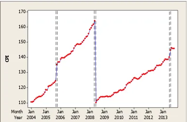
This study uses CPI of education, recreation, and sportdata in Indonesia. They are the monthly indexof 118 period from January 2004 to October 2013. To model the CPI data, the first step is the identification of the model inputsby observing time series and ACF plots. Figure 1. presents the time series plot of CPI data and Figure 2. presents the ACF plot of CPI data.

Year Month

2013 2012 2011 2010 2009 2008 2007 2006 2005 2004

Jan Jan Jan Jan Jan Jan Jan Jan Jan Jan 170

160

150

140

130

120

110

C

P

I

Figure 1.The time series and ACF plots of CPI data

30 28 26 24 22 20 18 16 14 12 10 8 6 4 2 1.0 0.8 0.6 0.4 0.2 0.0 -0.2 -0.4 -0.6 -0.8 -1.0

Lag

A

u

to

k

o

re

la

s

i

Here, we put two models which are differed from the inputs design. The inputs of the first FFNN modelareestablished based onthe ACFplotin Figure 2. The autocorrelationsare significant at lag 1, 2, 3, 4, 5, and6, so the inputs of FFNN are yt1, yt2, yt3, yt4, yt5, and yt1.This model is denoted as the FFNN1 model. The inputs of second model FFNN2 are formed by regarding the points where the data change drastically. From Figure 1.we can see that the data increase dramatically in the periods 21, 22, 53, 54, 113, and 114. Those points are referred to as knot points in truncated polynomial spline regression (TPSR) term. The pattern of data between knot points tend to rise. Thus, we generate 7 inputs of FFNN2 based on model (2) and (3), those are t0,

t1,t2, t3,t4,t5, and t6,

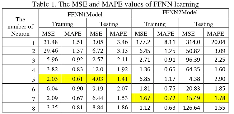
Then the step is continued to cross validation process by splitting the data into training and testing set. The training data start from period 1 to period 84, and rest are the testing data. Learning is done to determine the number of hidden neurons by considering the least MSE and MAPE values of training and testing data. Those values are presented in Table 1.

Table 1. The MSE and MAPE values of FFNN learning

The number of

Neuron

FFNN1Model FFNN2Model

Training Testing Training Testing

MSE MAPE MSE MAPE MSE MAPE MSE MAPE

1 31.48 1.51 3.05 3.46 177.2 8.11 314.0 20.04

2 29.46 1.37 6.72 3.13 6.45 1.25 50.82 3.09

3 5.96 0.92 2.57 2.11 2.71 0.91 96.39 2.25

4 3.82 0.83 12.0 1.92 1.36 0.65 64.35 1.60

5 2.03 0.61 4.03 1.41 6.85 1.17 4.38 2.90

6 6.04 0.90 9.19 2.07 1.81 0.75 20.83 1.85

7 2.09 0.67 6.44 1.53 1.67 0.72 15.49 1.78

8 3.35 0.81 8.84 1.86 1.12 0.63 126.64 1.55

The results in Table1. shows that the models with high degree of accuracy are FFNN1 models with 5 neurons and FFNN2 with 7 neurons in the hidden layer.

The next step is doing learning again to determine the optimal inputs. The combinations of inputs having the least MSE and MAPE values lead to the optimal model.The result of this step are given in Table 2.

Tabel2. The MSE and MAPE values of FFNN learning

FFNN1 Model Model FFNN2

Input (lag)

Training Testing

Input

Training Testing

MSE MAPE MSE MAPE MSE MAPE MSE MAPE

2, 3, 4, 5, 6 3.85 1.04 29.19 2.51 t1, t2, t3,t4,t5,t6 8.39 1.61 4620.0 3.98

1, 3, 4, 5, 6 3.97 0.80 8.62 1.83 t0, , t2, t3,t4,t5,t6 1.78 0.73 67.30 1.81

1, 2, 4, 5, 6 2.03 0.66 4.34 1.51 t0, t1,, t3,t4,t5,t6 1.73 0.69 87.74 1.71

1, 2, 3, 5, 6 21.06 1.61 46.45 3.69 t0, t1, t2, t4,t5,t6 3.55 0.89 37.66 2.21

1, 2, 3, 4, 6 16.78 1.41 4.09 3.24 t0, t1, t2, t3,t5,t6 3.12 0.89 41.56 2.21

1, 2, 3, 4, 5 3.02 0.83 23.70 1.91 t0, t1, t2, t3,t4,t5 1.55 0.66 90.10 1.63

1, 2, 3, 4,5 ,6 2.03 0.61 4.03 1.41 t0, t1, t2, t3,t4,t5 3.38 0.93 18.17 2.29

Table 2. demonstrate that the best models of FFNN1 is model with inputs lag1,2,4,5, and 6, and with 5 hidden neurons, and best models of FFNN2 is model with inputs t0, t1, t2, t3,t4,t5, t6, and with 7 hidden neurons.

Finally, the model fit is checked from residual ACF plot. Those of the models are delivered in Figure 3.

20

5% significance limits for the autocorrelations

20

5% significance limits for the autocorrelations

Figure3. The ACF plots of FFNN1and FFNN2residual

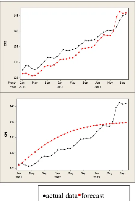
Furthermore, we also can explore the performance of the model from the plot of forecasts and actual data in training as well as in testing data.Figure 3. gives the plots for the training data and Figure 4. gives the plots for testing data.

2010 2009

2008 2007

2006 2005

2004

Jan Jan

Jan Jan

Jan Jan

Jan 170

160

150

140

130

120

110

C

P

I

2010 2009 2008 2007 2006 2005 2004

Jan Jan Jan Jan Jan Jan Jan

170

160

150

140

130

120

110

C

P

I

Figure 3.The time series plot of actual data and forecasts of FFNN1 and FFNN2 in training data.

Year Month

2013 2012

2011

Sep May Jan Sep May Jan Sep May Jan 145

140

135

130

125

C

P

I

2013 2012

2011

Sep May Jan Sep May Jan Sep May Jan 145

140

135

130

125

C

P

I

Figure 4 .The time series plot of actual data and Forecasts of FFNN1 and FFNN2 in testing data.

We can see that the plots of the forecastsand actual data in training data coincide. This fact demonstrate that all models yield accurate forecasts. Meanwhile, only the plot of FFNN1 show good performance in testing data. The plot of FFNN2hasexponential trend, which is very different from the pattern of the actual data. So, we recommend the FFNN1 to be the optimal model for CPI of education, recreation, and sport datain Indonesia.

Conclusion

The CPI of education, recreation, and sport in Indonesia has an upward trend and has many jump points. So, here we examines the modelswith two possible input design, those are inputs generated from the lags of variableand the inputs such as in the TPSR model.The result shows that the best model is FFNN models with inputsgenerated fromthe lags of variables. This model deliver high accuracy both in training and testing data.

Refference

Chen X., Racine J., and Swanson N. R. (2001). Semiparametric ARX Neural-Network Models with an Application to Forecasting Inflation. IEEE Transaction on Neural Networks, Vol. 12, No. 4, pp. 674-683.

Cybenko, G. (1989). Approximation by Superpositions of a Sigmoidal Function. Mathematics of Control, Signals and Systems, Vol. 2, pp. 304–314.

Funahashi, K. (1989). On the approximate realization of continuous mappings by neural networks. Neural Networks, 2, 183–192.

Hornik K. (1989). Multilayer Feedforward Networks are Universal Approximation. Neural Networks, 2, 359 – 366.

HaykinS. (1999). Neural Networks, A comprehensive foundation, Ontario:Pearson Education.

Suhartono, Subanar, Rejeki S. (2005). Feedforward Neural Networks Model for Forecasting Trend and Seasonal Time series. IRCMSA Proceedings. Sumatra Utara Indonesia.

Wei, W.W.S. (2006). Time Series Analysis, Univariate and Multivariate Methods, 2nd ed. New York: Pearson.

Wand M. P. (2000). “Comparison of regression spline smoothing procedures,”

Computational Statistics, 15, 443- 462.

Wutsqa D.U. (2005). Comparison between the Neural Network (NN) and ARIMA Models for Forecasting the inflation in Yogyakarta. Proceeding ICAM, ITB, Bandung.

Wutsqa D.U. and Abadi A. M. (2011). Modeling Islamic Lunar Calendar Effect in Tourism Data of Prambanan Templeby Using Neural Networks And Fuzzy Models. Presented in ICCT, Nidge, Turkey.

Wutsqa D.U. and Yudhistirangga, “Modeling consumer prices index data in

Yogyakarta using truncated polynomial spline regression,” Proceeding SEACMA, ITS, Surabaya, 2013.