Full Terms & Conditions of access and use can be found at
http://www.tandfonline.com/action/journalInformation?journalCode=ubes20
Download by: [Universitas Maritim Raja Ali Haji] Date: 12 January 2016, At: 23:48
Journal of Business & Economic Statistics
ISSN: 0735-0015 (Print) 1537-2707 (Online) Journal homepage: http://www.tandfonline.com/loi/ubes20
A Discrete-State Continuous-Time Model of
Financial Transactions Prices and Times
Jeffrey R Russell & Robert F Engle
To cite this article: Jeffrey R Russell & Robert F Engle (2005) A Discrete-State Continuous-Time Model of Financial Transactions Prices and Times, Journal of Business & Economic Statistics, 23:2, 166-180, DOI: 10.1198/073500104000000541
To link to this article: http://dx.doi.org/10.1198/073500104000000541
Published online: 01 Jan 2012.
Submit your article to this journal
Article views: 178
View related articles
A Discrete-State Continuous-Time Model of
Financial Transactions Prices and Times:
The Autoregressive Conditional Multinomial–
Autoregressive Conditional Duration Model
Jeffrey R. R
USSELLGraduate School of Business, University of Chicago, Chicago, IL 60637 (jeffrey.russell@gsb.uchicago.edu)
Robert F. E
NGLEStern School of Business, New York University, New York, NY 10012 (rengle@stern.nyu.edu)
Financial transaction prices typically lie on a discrete grid of values and arrive at random times. This paper proposes an econometric model with this structure. The distribution of each price change is a multinomial, conditional on past information and the time interval between the transactions. The proposed autoregres-sive conditional multinomial (ACM) model is not restricted to be Markov or symmetric in response to shocks; however, such restrictions can be imposed. The duration between trades is modeled as an autore-gressive conditional duration (ACD) model following Engle and Russell (1998). Maximum likelihood estimation and testing procedures are developed. The model is estimated with 12 months of tick data on a moderately frequently traded NYSE stock, Airgas. The preferred model is estimated, with three lags for the ACM model and two lags for the ACD model. Both price returns and squared returns influence future durations and present and past durations affect price movements. The model exhibits reversals in transaction prices in the short run due to bid–ask bounce and clustering of large moves of either sign in the longer run. Evidence of symmetry in the dynamics of prices is seen, but the response to durations is clearly nonsymmetric. It is found that the volatility per second of trades is highest for short-duration trades and that expected returns are lower for longer-duration trades.
KEY WORDS: Autoregressive conditional duration; Bid–ask bounce; Discrete-valued time series; High-frequency data; Marked point process; Markov chain; Multinomial; Transaction price.
1. INTRODUCTION
The role of computers in modern business has generated a new type of economic data where every single transaction is recorded. Nowhere is this refinement in data collection more ex-tensive than for financial data, where transaction-by-transaction datasets contain detailed information about precisely when an asset is traded, as well as such characteristics as the transac-tion price and quantity. These new datasets provide us with an unprecedented microscopic view of the structure of financial markets that was previously impossible with time-aggregated data.
Econometric modeling of transaction-by-transaction price dynamics is complicated by several features of the data. First, in a continuous auction market, such as the NYSE or the NASDAQ, transactions can occur at any point in time that the market is operational. As such, transactions do not occur at regularly spaced time intervals. The times between trades are random and are potentially informative about the underlying processes. Second, every financial market structure specifies a minimum unit of price measurement, called a tick. That is, transaction prices must fall on a grid. When viewed over long time horizons, the variance of price changes greatly exceeds the effects of discreteness, so that treating the data as continuous is unlikely to have a meaningful impact on the analysis. At the transaction-by-transaction frequency, however, price discrete-ness becomes a dominant feature of the data. Institutional rules for a given market determine the granularity of the
discrete-ness. Often institutional rules in markets restrict the number of ticks that the price can move from one transaction to the next. In the NYSE this is done by the specialist responsible for “price continuity.” In other electronic markets, like the Taiwan stock exchange, price restrictions are directly imposed by so that consecutive prices can differ by no more than a fixed num-ber of ticks. Hence the observed price changes often take just a handful of values. For the transactions data studied in this ar-ticle, for example, we find that 99.3% of the price changes fall on one of just five different values.
An econometric model of such a process must be a conti-nuous-time process in that it should give at every instant of time the probability of observing a transaction at a particular discrete price, conditional on the past history of these processes. Most econometric models are not capable of this task and proceed by first converting to calendar time and then ignoring the discrete-ness of prices. Any such procedure inevitably involves a loss of information and frequently leads to bias.
In this article we propose a new approach to modeling high-frequency transaction price dynamics that addresses both the spacing and the discreteness of the data. We propose treating the transactions data as a sequence of arrival times and charac-teristics associated with those arrival times. This is commonly
© 2005 American Statistical Association Journal of Business & Economic Statistics April 2005, Vol. 23, No. 2 DOI 10.1198/073500104000000541 166
known as amarked point processin the statistics literature. Fol-lowing Engle (2000), we decompose the joint distribution into the product of the conditional distribution of price changes and the marginal distribution of the time interval. We propose us-ing a variation of the autoregressive conditional duration (ACD) model of Engle and Russell (1998) for the marginal distrib-ution of arrival times. We then propose a new model for the discrete price movements that is flexible enough to capture the complex temporal dependence typically displayed by high-frequency transactions data. We call this model the
autoregres-sive conditional multinomial(ACM) model.
Although the proposed ACM model seems particularly well suited for analysis of financial transactions data, or movements in the midpoint of the discrete bid and ask quotes, it could also be useful in many other applications involving time series of discrete random variables. For example, traders face a fixed number of possible order flow strategies involving market or-ders versus limit oror-ders. The model may be useful in the study of the dynamics of order flow without the need to impose a Markovian structure. Alternatively, the ACM model may prove useful for credit risk ratings in financial markets or in market-ing, where product brands purchased by consumers over time are of interest. The model can be applied to fixed-interval data or, if the time series is viewed at irregular intervals, jointly mod-eled using the durations and the discrete random variable of in-terest. Hence, although the immediate application is to financial transactions data, we believe that the model could prove useful various other settings.
We apply the model to an NYSE-traded stock. Given the joint distribution, we can examine the nature of the depen-dence between contemporaneous durations and transaction price changes. Two strands of theoretical market microstructure models provide predictions regarding the nature of dependence between transaction rates and price adjustments. First, Easley and O’Hara (1992) suggested that high trading rates may be associated with the presence of informed traders. In a ratio-nal expectations setting, the specialist will make price adjust-ments more sensitive to order flow, thereby increasing volatility. Hence rapid trading should be associated with higher volatility. Second, Diamond and Verrecchia (1987) suggested that short sale constraints restrict the ability of privately informed agents possessing “bad news” to transact and capitalize on their better information. Because no such restraints exist in long positions, high trading rates tend to be associated with good news and ris-ing prices, whereas the converse is true for slow tradris-ing rates.
We estimate the preferred model with three lags for the ACM and two lags for the ACD. Both price returns and squared re-turns influence future durations, and present and past durations affect price movements. The model exhibits reversals in trans-action prices in the short run due to bid–ask bounce and cluster-ing of large moves of either sign in the longer run. We present evidence of symmetry in the dynamics of prices, but, consis-tent with the theory of short sale constraints and information of Diamond and Verrecchia (1987), we find that the response to durations is clearly nonsymmetric, with long durations predict-ing fallpredict-ing prices. Consistently with the results of Easley and O’Hara (1992), we find that the volatility per second of trades is highest for short-duration trades and that expected returns are lower for longer-duration trades. Finally, we find that both price changes and squared price changes influence future durations.
The article is organized as follows. Section 2 discusses the general modeling approach for irregularly spaced, discrete valued transactions data advocated in the article. Section 3 introduces the ACM model for the discrete price changes, de-velops some theoretical properties of the model are developed, and presents estimation and model diagnostics. It also consid-ers parameter restrictions for the ACM model derived from a symmetry condition. Section 4 presents model estimates and analysis for an NYSE-traded stock, and Section 5 concludes.
2. AN APPROACH TO JOINT MODELING
OF ARRIVAL TIMES AND PRICE CHANGES
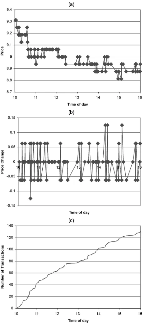
The modeling strategy that we adopt is conveniently mo-tivated by first considering a short, representative sample of trades for the NYSE-listed stock Airgas (ARG). In Figure 1(a) the calendar time (or clock time) is on the horizontal axis and the price is on the vertical axis. Each diamond represents a point in time that a transaction occurred and the associated price. Two features of the data immediately become apparent. First, the in-tertrade durations vary significantly within the sample, as can be observed in the plot by noting the occasional long horizon-tal stretch between observations. Second, the transaction price changes take just five different values in this sample. Hence price discreteness is a dominant feature of the data.
We propose decomposing the time series plotted in Fig-ure 1(a) into a bivariate system. This is shown graphically in Figures 1(b) and 1(c). Figure 1(b) presents the discrete price changes from transaction to transaction. Figure 1(c) presents the counting function that denotes the number of transactions that have occurred by timet. These series make up the bivari-ate system. More formally, lettidenote the arrival time of the
ith transaction. LetN(t)denote the counting function that de-scribes the number of events that have occurred by timet. A se-quence of arrival times that are strictly increasing is called a
simple point process. At each transaction time ti, we denote
the associated realization of the trade-to-trade change in the asset price by yi. The bivariate process of arrival times and
marks is called a marked point process. Because transaction price changes are typically discrete in nature, we consideryto be a multinomial random variable.
A simple point process can be completely described by the sequence of arrival times, ti, or the durations, τi =ti−ti−1. Our goal is to develop a model for the joint distribution of the discrete price changes and durations conditional on the bivari-ate filtration of arrival times and price changes. We denote this conditional bivariate density by f(yi, τi|y(i−1),τ(i−1)), where
y(i−1)=(yi−1,yi−2, . . . ,y1) andτ(i−1)=(τi−1, τi−2, . . . , τ1). Our discussion entails a substantial use of superscripts and subscripts. (See Appendix A for a summary of the super-script/subscript notation.)
As discussed by Engle (2000), without any loss in generality we can decompose the joint conditional density of yi and τi
into the product of the conditional density of the mark and the marginal density of the arrival times, both conditioned on the past filtration of the joint information set. That is, if f(yi, τi)
(a)
(b)
(c)
Figure 1. One Day of Transactions Data. (a) Transaction price; (b) transaction price changes; (c) number of transactions that have oc-curred.
whereg(·)denotes the probability density function associated with the price changesyiconditional onτ(i)andy(i−1), andq(·)
denotes the density function of theith duration conditional on τ(i−1) andy(i−1). Clearly, the joint density in (1) allows us to study the relationship between price changes and contempora-neous durations, as well as analyze their joint dynamics.
Models that explain the probability of each possible out-come of a discrete random variable at timeτ, are often called
competing-risks models (see Kalbfleish and Prentice 1980;
Lancaster 1990 for references on duration models). The joint density in (1) clearly yields such a set of probabilities.
Com-peting risks models are generally specified by the instantaneous probability of exit to stateygiven a durationτ. The hazard func-tion denoting the instantaneous probability that theith trade ex-its to stateygiven the durationτ since the last event,
θi(y, τ )
= lim
t→0
Pr(Yi=y, τ≤τi< τ+t|τi≥τ,y(i−1),τ(i−1))
t .
(2)
For small values of t, θi(y, τ )t is approximately equal to
the probability of exit to stateyover the time period[t,t+t]
given that no transaction has occurred by durationτ. The hazard functions are easily obtained from (1) and are given by
θi(y, τ )=κτ
y(i−1)τ(i−1)
gyy(i−1),τ(i)
, (3)
where κ(τ|y(i−1),τ(i−1)) = q(τ|y(i−1),τ(i−1))/(1 − τ
0 q(s|
y(i−1),τ(i−1))ds)is the hazard function associated with the
dis-tribution of the waiting times between transactions.
Clearly, conditional moments of the price changes can be ob-tained directly from (1). Moments of price changes and trad-ing rates over more than one transaction can sometimes be expressed analytically, but calendar time measures will gener-ally require simulations.
Instantaneous moments of the price process are also easily obtained. We define the price at timetas the price associated with the most recent transaction and denote it byp(t)=p(tN(t)).
The instantaneous mean and variance of the price change at timetcan be conveniently expressed using the counting func-tionN(t)as
µ(t)= lim
t→0
E((p(t+t)−p(t))|N(t),y(N(t)),t(N(t)))
t
=
ally
yθN(t)y,t−tN(t) (4)
and
σ2(t)
= lim
t→0
E{[(p(t+t)−p(t))−µ(t)]2|N(t),y(N(t)),t(N(t))}
t
=
ally
y2θN(t)y,t−tN(t)−(µ(t))2. (5)
The instantaneous moments conveniently characterize the evo-lution of the price process. All else being equal, the magnitude of the instantaneous mean and variance will be larger when the probability of a transaction is higher.
Engle and Russell (1998) proposed the ACD model forq(·)
and found that the model performs well for transactions data. A wide range of empirical studies have now compared various specifications of this general ACD form (see, e.g., Bauwens, Giot, Grammig, and Veredas 2003). Given an ACD formula-tion forq(·), the only remaining task is to specify a model for the pricesg(·). We now focus our attention on modeling the conditional distribution of price changesg(·).
3. THE AUTOREGRESSIVE CONDITIONAL MULTINOMIAL MODEL
Unlike their low-frequency counterparts, high-frequency price changes tend to exhibit strong and often complex tem-poral dependence. Any good model for the price changes thus must be flexible and capable of generating strong dependence spanning many transactions. In this section we develop a time series model for discrete random variables consistent with this goal, the ACM model. We also establish some theoretical prop-erties for an ACM model.
3.1 Model Specification
Many models have been suggested in the context of parame-ter-driven models and associated hidden Markov models. Al-though this literature is rich, the models are often difficult to estimate and forecast. (See MacDonald and Zucchini 1997 for a recent survey of these models.) Relatively little work has been done on discrete-valued observation-driven models in the sense of those of Cox (1981). Jacobs and Lewis (1983) pursued a class of models for discrete-valued time series data called DARMA models. But these models often have unrealistic properties, such as nonnegative autocorrelation restrictions. Furthermore, they appear better suited for marginally Poisson or binomial data. Our proposed ACM model is applicable to multinomial data.
Here we restrict our attention to the class of observation-driven models. Let k denote the number of states that the multinomial random variable yi can take. Let x˜i be a k×1
vector indicating the discrete price change yi; x˜i takes the jth
column of thek×kidentity matrix if the jth state occurred. Letπ˜i denote thek×1 vector of conditional (on information
available at timeti−1) probabilities associated with the states. That is, thejth element ofπ˜icorresponds to the probability that
thejth element ofx˜itakes the value 1. Clearly, the conditional
distribution ofyi is completely characterized byπ˜i. A natural
starting point is a Markov chain. A first-order Markov chain can be expressed as
˜
πi=Px˜i−1, (6) wherePis ak×ktransition matrix that must satisfy that (a) all elements are nonnegative and (b) all columns must sum to unity. In the more general setting,Pmay be a conditional transi-tion matrix and will vary with informatransi-tion available at period
(i−1). In this context, we can include information on longer lags ofx˜, perhaps past values ofπ˜ and the past arrival times of the transactions. An early discussion of time-varying tran-sition probabilities was given by MacRae (1977), although the emphasis there was on estimation when only aggregate data are available.
The restrictions onPare directly satisfied by simple estima-tors when the transition matrix is constant, but become quite difficult to impose in simple extensions. Here we propose using an inverse logistic transformation that imposes such conditions directly for any set of covariates.
Letπimandxijdenote themth andjth elements ofπiandxi.
constant. [Henceforth, vectors with tildes denotek-dimensional vectors and, unless otherwise specified, vectors without a tilde denote(k−1)-dimensional vectors.] Rewriting thek−1 prob-abilities as the vectorπ, and defining the vector of logs of the probability ratios as h(πi)=log(πi/(1−ι′πi)), whereι is a
conforming vector of 1’s, we get
h(πi)=P∗xi+c, (8)
whereP∗ is an unrestricted(k−1)×(k−1)matrix andcis a(k−1)vector withmth element given bycm. For any values
of P∗ andc, the conditional probabilities are easily recovered from the logistic transformation
where againιdenotes a conforming vector of 1’s and exp(P∗)
is interpreted as a matrix withm,nelement exp(P∗mn). Now all probabilities will be positive, including the probability of the
kth state are obtained from condition (b) and will sum to unity. An expression for the transition probabilities is then obtained,
Pmn=
exp[P∗mn+cm]
1+k−1
j=1exp[P∗jn+cj]
, (10)
and again these are all positive and have columns that sum to unity.
We now consider generalizing (8) to allow for a more elabo-rate dynamic structure with dependence on a richer information set than just the most recent price movement. In doing so, it is clear that we are generalizing the transition matrix in (2) from a time-invariant transition matrix to one that varies over time.
Definition 1. An ACM model of order(p,q)is given by
(r+1)-dimensional vector with 1 in the first element forming a constant andr other explanatory variables, andχ denotes a
(k−1)×(r+1)conforming matrix of parameters. These ex-planatory variables may contain predetermined variables, such as characteristics of past trades including volume or spreads, or, as of interest in our application, the vector zmay include
information about the timing of trades. The terms (xi−πi)
form a martingale difference sequence characterizing the new information associated with theith transaction. In an interesting working paper, Shephard (1995) considered generalized linear autoregressive time series models in the same spirit as (7).
Clearly, (11) can be interpreted as specifying dynamics for the conditional log odds for all states with respect to a base state and therefore specifies the dynamics of the conditional log odds for all pairs of states. It follows that the specifica-tion in (11) completely describes the transispecifica-tion probabilities and hence the dynamics of the multinomial random variableyi. The
linear structure of (11) implies that the choice of the base state is arbitrary. This is easily verified because parameters for the choice of any base state can be expressed as an exact function of the parameters of any other choice of base state.
From (11), it is immediately apparent how the history im-pacts the transition probabilities. The structure of this equation is recursive. At the time of the i−1 transaction, knowing all past xandπ gives from (9) a calculated value of the nextπ. Consequently, subject to some starting values, the full sequence of transition probabilitiesπ can be constructed from observa-tions on x. This allows evaluation of the likelihood function and its numerical derivatives. It can now be seen that the first
(k−1)-conditional probabilities are easily recovered from
πi=exp
Thekth probability is determined by condition (b). Hence the transition probabilities are given byπi, and the conditional
co-variance matrix ofxcan be defined as
Vi≡V
We now turn to some theoretical properties of the model. For illustrative purposes, consider the ACM(1,1)model whenp=
q=1 andr=0, so that zi is simply a constant denoting the
intercept. When the eigenvalues ofBare distinct and lie inside the unit circle, we can rewrite the ACM(1,1)model as
a martingale difference sequence, the dynamics of the ACM model are easily understood from (14). The impact of past in-formation is determined byA, whereas the decay of past infor-mation is determined by the eigenvalues ofB. Generalizing (14) to an ACM(p,q), we can construct bounds for the transition probabilities determined by the parameters of the ACM model. These results are summarized in the following theorem.
Theorem 1. Consider the ACM(p,q) model given by (11)
withr=0 (denoting a constant term only), and let theAi (i=
1, . . . ,p)andBj(j=1, . . . ,q)be of full rank. LetIk−1denote the(k−1)-dimensional identity matrix. If all of the values ofz
satisfying|Ik−1−B1z−B2z2− · · · −Bqzq| =0 lie outside the
unit circle, then the elements ofπiare strictly positive.
For the proof see Appendix B.
Corrollary 1. Under the conditions of Theorem 1,yiis
irre-ducible, meaning that regardless of the initial condition, every state will be visited infinitely often asi→ ∞. Furthermore,yis aperiodic in the sense that the minimum recurrence time is one period.
Proof. This follows trivially from Theorem 1 and the fact
thatkis finite.
Corrollary 1 ensures that in the long run, all states will be visited infinitely often and that the transition matrix will always be fully saturated; that is, any state is attainable regardless of the sequence of preceding price moves. It would seem that any good model for the transition probabilities of transaction prices should have these properties. We note that Theorem 1 does not necessarily provide sufficient conditions for stationarity of the transaction price process.
It should be noted that Hausman, Lo, and Mackinlay (1992) have proposed modeling discrete price changes using a probit model with time-varying mean and variance. But their approach allows for very limited dependence due to its Markov structure and is far less flexible regarding the impact of new information on the transition probabilities.
3.2 Estimation and Diagnostics for the ACM Model
Given initial conditions, the entire path of πi can be
con-structed. Hence the likelihood can be constructed as the product of the conditional densities. Lettingπij denote thejth element
ofπithe log-likelihood is then expressed as
L= likelihood take a recursive form analogous to those of gener-alized autoregressive conditional heteroscedasticity (GARCH) models. We therefore propose estimating the model by maxi-mum likelihood using a numerical optimization algorithm such as that of Berndt, Hall, Hall, and Hausman (1974) (BHHH here-after). Under the usual regularity conditions, we obtain consis-tent asymptotically normal parameter estimates.
Model diagnostic tests are suggested by considering the se-quence of errors
v∗i =xi−πi. (16)
This sequence should form a heteroscedastic martingale differ-ence sequdiffer-ence, where the conditional variance–covariance ma-trix is given byVi in (13). Standardized errors are constructed
by premultiplyingv∗i by the Cholesky factorization of the con-ditional variance–covariance matrix. The standardized errors are given by
vi=Uiv∗i, whereUiViUi=I. (17)
Now νi should be uncorrelated with the past and have a
variance–covariance matrix equal to the(k−1)identity matrix. Moreover,νi should be uncorrelated with the filtration of price
moves and any information inzi. Given parameter estimates, we
can construct the series of standardized residuals,vˆi, the
sam-ple counterpart to (17). We can then be perform tests to check whether vˆi is uncorrelated. Thesth sample cross-correlations
associated with the standardized residuals are calculated by
Ps=
1
N−(s+1)
N
i=s+1 ˆ
vivˆ′i−s. (18)
A formal test of the null hypothesis that the elements of the standardized vector are white noise can be done with a mul-tivariate version of the Portmanteau statistic. Li and McLeod (1981) proposed a test based on the statistic
Q=N
M
s=1
Trace(PsP′s). (19)
This test statistic will be distributed as a chi-squared distribu-tion with(k−1)2×Mdegrees of freedom.
3.3 Symmetry in Price Dynamics
In this section we propose some parameter restrictions for the general ACM(p,q) model. Harris (1990) provided a de-tailed discussion of the effects of price discreteness on esti-mates of autocorrelations (and the variance) calculated from the observed return series. The cornerstone of Harris’ work is the idea that the observed transaction price is the “true” price of the asset plus an upward (downward) departure for buyer (seller) initiated trades rounded to the nearest tick. Harris as-sumes that the arrivals of buyers and sellers can be described by an iid Bernoulli with constant probability .5. If order flow is correlated, as was suggested by Hasbrouck (1991), then analy-sis of the effects of discreteness on the price dynamics becomes much more complicated. In the presence of (unobserved) time-varying risk, the magnitude of departures of the observed price from the efficient price may also be time-varying, further com-plicating any analysis of the price dynamics. In this more real-istic setting, we have little theory to guide us in determining the dynamics of discrete bid and ask prices.
Nevertheless, there is a particular type of symmetry that we might expect in the dynamics of the price movements. This hy-pothesis is most easily understood by examining a simple spe-cial case. Consider the simple two-state time-invariant Markov model given in (6). Let state 1 denote a downward price move-ment and state 2 denote an upward price movemove-ment, and let
pij denote thei,jth element ofP. Our symmetry hypothesis
re-strictsp12=p21 andp11=p22. These restrictions impose that the probability of a price continuation is the same regardless of whether the price is moving up or down. Similarly, the probabil-ity of a price reversal is the same regardless of whether the price moved up or down. Following state 1, the conditional distribu-tion is[p11p21]′ and, imposing the foregoing restrictions, the conditional distribution following a downward price movement is given by[p21p11]′. The restrictions imply that the conditional distribution following an upward (downward) price move is the
mirror image of the conditional distribution following a down-ward (updown-ward) price move, and vice versa.
We now generalize the symmetry hypothesis beyond the sim-ple first-order Markov model and to more than just two states. Define the matrixQto be a rotated identity matrix,
Q=
0 1
. ..
1 0
. (20)
The elements of a conforming vector are reversed when premul-tiplied byQ. Arrangexi in the natural ordering, with the first
element corresponding to the extreme downward price move and the last element corresponding to the extreme upward price move. The zero price move is taken to be the base state given by the zero vector. We define the mirror-image history by Qxi−1,
Qxi−2, . . .; that is, upward price movements become down-ward price movements of equal magnitude in the mirror im-age. For a general k-state model with (k−1)/2 upward price movement states and corresponding (k−1)/2 downward price movement states, we state the following definitions.
Definition 2. An n×n matrix Wis response-symmetric if
for the n×n matrix Qdefined in (16), QW=WQ; that is,
QandWcommute.
Definition 3. A vectorwis symmetric ifQw=w.
Definition 4. For an ACM(p,q) model, we say the
trans-action price process is dynamic-symmetric for prices if all
AiandBiare response-symmetric matrices.
Definition 5. For an ACM(p,q)model, we say that the
trans-action price process is dynamic-symmetric for thejth element ofziif thejth column ofχis a symmetric vector.
In this case the marginal impact of a dynamic-symmetric el-ement ofzon the log odds is the same for price moves of equal but opposite direction.
Proposition 1. If an ACM(p,q)model is
dynamic-symmet-ric for pdynamic-symmet-rices and elements ofZ, thenQπi(xi−1,xi−2, . . . ,zi)=
πi(Qxi−1,Qxi−2, . . . ,zi).
For the proof see in Appendix B.
When xi arranged in its natural ordering, the conditions
of Proposition 1 imply that the mirror-image history of price changes will produce the mirror-image transition probabilities. When the ACM model is dynamic-symmetric for prices but not for all elements ofz, there is a remaining symmetry in the mar-ginal impacts of the past price changes on the log odds of the transition probabilities.
Proposition 2. Let Hs denote a matrix with m,n element
given bydhim/dxi−s,n, wheremandndenote themth andnth
elements of h and x. If an ACM(p,q) model is dynamic-symmetric for prices, thenHs is a response-symmetric matrix
for alls>0.
For the proof see Appendix B.
The implications of Proposition 2 are most easily understood by returning to the simple two-state model described earlier. Proposition 2 says that the marginal impact of a downtick on the log odds of a subsequent uptick is identical to the marginal
impact of an uptick on the log odds of a subsequent downtick. Similarly, the marginal impact of an uptick on a subsequent uptick is identical to the marginal impact of a downtick on a subsequent downtick. If an ACM(p,q)is dynamic-symmetric for prices and the constant is a symmetric vector, then the num-ber of parameters is reduced from(k−1)(1+(k−1)(p+q))
to (k−21)(1+k(p+q)), or by almost half. Clearly, this restric-tion can be tested in practice.
A final model restriction that we consider is to set off-diagonal elements of allBjto 0. Under this assumption, the
par-tial derivative of the log odds with respect to a unit shock will decay at a geometric rate determined by the diagonal elements of the Bj. Thus the impact of new information is generously
specified, whereas the long-run decay is more parsimoniously formulated. We refer to this restriction as thediagonal
specifi-cation.
4. DATA AND ESTIMATION
In this section we provide a description of the financial trans-action data and consider estimation and diagnostic tests of an ACM–ACD model. We also present tests for the symmetry hy-pothesis discussed in Section 3.3. On finding a good representa-tion for the data, we analyze the nature of dependence between transaction price changes and durations. Our findings are re-lated to predictions obtained from existing market microstruc-ture theory. We begin with a more detailed discussion of the data.
4.1 Data
The number of transactions per day varies greatly from stock to stock. For example, IBM may experience 10,000 transac-tions in a single day (or about a trade every 2 or 3 seconds), whereas other stocks trade very infrequently, often going an en-tire day without any transactions. We try to strike a balance in this application by selecting a stock that trades about once every 3 minutes on average. This trading frequency provides a large number of transactions per day, but remains tractable enough to analyze 1 complete year of data. The stock that we analyzed is Airgas (ticker symbol ARG). This is the first stock alphabet-ically in decile 8 of the stocks examined by Engle and Patton (2003). Their selection was based on trade frequency during the previous year, with decile 10 as the most frequently traded stocks. The data used in this article were abstracted from the TAQ (Trades and Quotes) dataset distributed by the NYSE.
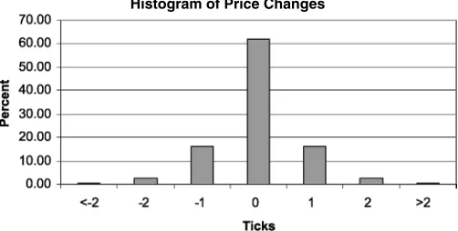
Over the 1-year period January–December 1999 there were 21,837 transactions. The average transaction price for the sam-ple is $10.44. The minimum price change for ARG during this period is 1/16th of a dollar. Following Engle and Rus-sell (1998), we omit the first half-hour of trades, because some of these will contain trades recorded during the opening batch auction. We also delete overnight price changes, leaving a sam-ple of 18,573 transactions, of which 61.72% of the transaction prices are unchanged from their previous value. The distribution of transaction price changes is roughly symmetric, with 16.20% down one tick and 16.36% up one tick. Down and up two ticks occurred with 2.60% and 2.39% frequency. Downward moves greater than two ticks occurred with frequency .30%,
Histogram of Price Changes
Figure 2. Histogram of Transaction Prices.
and upward moves greater than two ticks occurred with fre-quency .41%. A histogram of the transaction price changes is presented in Figure 2, and the raw frequencies are given in Ap-pendix C.
Given the sparseness of the data beyond two tick moves, we use a five-state model. The two extreme states therefore include upward price movements of two or more ticks and downward price movements of two or more ticks. We use the natural or-dering for the state vector given by
xi=
[1,0,0,0]′ ifpi≤ −2 ticks [0,1,0,0]′ ifpi= −1 tick [0,0,0,0]′ ifpi=0 [0,0,1,0]′ ifpi= +1 tick [0,0,0,1]′ ifp
i≥ +2 ticks.
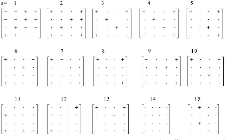
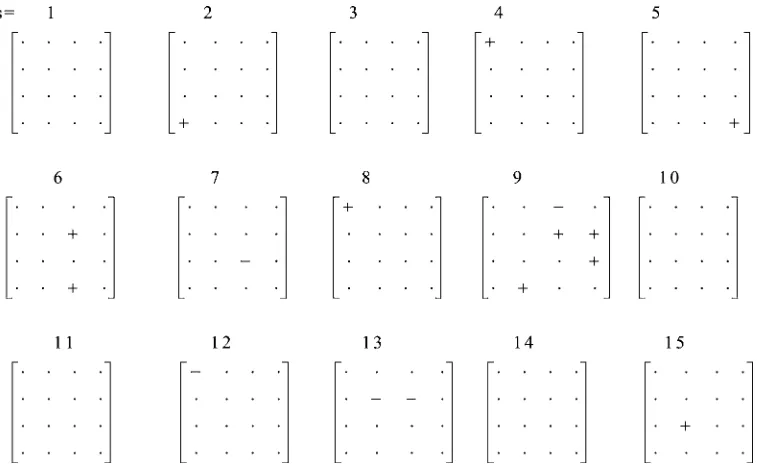
The state vector provides an interesting perspective from which to view the dynamics of the transaction price changes. Using the multivariate summary methodology initially pro-posed by Tiao and Box (1981), the intertemporal cross-correla-tions of the state vector are presented in matrix form, with the correlations replaced by the symbols “+,” “−,” and “·.” If the price changes were iid, then an asymptotic 95% confidence in-terval would be given by 1.96×N−1/2. A dot indicates that a correlation does not exceed this 5% significance level. Plus and minus signs indicate positive and negative exceedences.
Denoting the sample mean ofxi by thek-dimensional
vec-torx¯, thesth sample cross-correlation matrix is calculated by
Ps=R−01Rs, where
Rs=
1
N−(s+1)
N
i=s+1
(xi− ¯x)(xi−s− ¯x)′. (21)
The Tiao–Box plot for the state vector temporal correlations up through lag 15 is given in Figure 3. Thei,jelement of the
sth matrix gives the correlation of state i with statej lagged
speriods. The upper right and lower left quadrants, correspond to price reversals; the upper left and lower right quadrants, to price continuations. Fors=1, the cross-correlations are gen-erally positive in the upper right and lower left quadrants, and negative in the upper left and lower right quadrants, indicating that price reversals are more likely than price continuations im-mediately after a price move. The transaction price “bounces” back and forth between buy and sell prices, generating negative autocorrelation in transaction price changes and the observed
Figure 3. Box–Tiao Representation of Sample Cross-Correlations ofx.Rs=N−(1s+1)iN=s+1xix′i−s,Ps=R
−1 0 Rs.
positive signs associated with the price reversals. This is often referred to asbid–ask bounce.
Beyond the first lag, the significant correlations are generally positive. Significant elements tend to occur most often in the corners of the matrix and sometimes in the center. This pattern implies that large price changes (of two or more ticks) tend to follow large price changes of either direction, and small price changes tend to follow small price changes of either direction. This pattern is an expression of volatility clustering in the dis-crete price moves.
Finally, we notice a particular symmetry in the correlations. For many of the correlations, the signs of the correlation re-flected through the origin are the same. If the symmetry condi-tions discussed in Section 4 are satisfied, this is the exact pattern the correlations should display. We formally test the symmetry condition later in this section.
The time intervals between trades are known to contain a pe-riodic U-shaped pattern throughout the trading day. Durations tend to be shortest in the morning just before the open and in the afternoon just before to the close. Intraday volatility also exhibits a similar periodic pattern, although this pattern is typi-cally examined using price data observed over fixed time inter-vals (see, e.g., Engle and Russell 1998 for diurnal patterns in
durations and McInish and Wood 1992 for an early analysis of volatility periodicity).
We examine the state vector xi to check for any evidence
of these diurnal effects in the distribution of transaction-by-transaction price movements. In doing, so we may detect, pat-terns in the variance or any other moments of the price changes, if present. We treat each of the four elements ofxias a
univari-ate time series and fit by least squares a linear spline in the time of day. Nodes are placed at each hour of the trading day, and the spline is restricted to be continuous. The result for thejth series is an estimate of the probability that statejoccurs at any point during the day. This parallels the two-step procedure that Engle and Russell (1995) used to estimate deterministic patterns. If there are no diurnal effects, the coefficients should be 0, with only the intercept non-0. AnF-statistic is provided to assess the null hypothesis that there are no diurnal effects. The estimates for the time-of-day effects for each price change state and the durations are given in Table 1. For each regression,djdenotes
thejth spline coefficient estimate.
From Table 1, we see that the durations tend to be shortest near the open and close of the market and longest in the mid-dle of the day; this is the inverted U-shape typically observed. Thepvalue for the null hypothesis of no time-of-day effects is
Table 1. Estimates of the Deterministic Pattern for Durations and States
Const. d1 d2 d3 d4 d5 d6 F-statistic p value
Durations 239.30 −16.84 65.20 43.08 −41.88 −63.26 −118.25 0% (11.83) (17.02) (14.24) (15.03) (15.10) (14.39) (17.69)
Down 2 .030 −.0034 .0083 0 −.0153 .00625 .00818 6.432% (.0053) (.0076) (.0064) (.0067) (.0067) (.0064) (.00795)
Down 1 .165 −.0077 .0060 −.0046 .00659 .00773 −.0292 61.3% (.0117) (.0168) (.0140) (.0148) (.0149) (.0142) (.0175)
Up 1 .156 .0147 −.0106 .0196 −.029 .0030 .0227 25.6% (.0117) (.0169) (.0141) (.0149) (.0149) (.0142) (.0175)
Up 2 .0395 −.0172 .0106 −.0042 −.0059 .0053 .0013 23.3% (.0052) (.0075) (.0063) (.0066) (.0067) (.0064) (.0078)
near 0, and the hypothesis is easily rejected for the durations. Alternatively, the price changes do not exhibit any indication of periodicity. The coefficients appear to be random with no real pattern, and all are insignificant. Thepvalue for the null of no time-of-day effects is large for all of the price states. The small-estpvalue is for state 1 (down two or more ticks), which has a
pvalue of 6.43%.
It is interesting to find no evidence of a deterministic pattern in the transaction-by-transaction price dynamics and particu-larly no pattern in the magnitude of the price changes, because periodicity in volatility patterns is well documented for intraday prices measured in fixed time intervals. This suggests that the time-of-day patterns discovered for volatility using within-day fixed-interval analysis are driven by time-of-day patterns in the transaction rates rather than by the magnitude of transaction-by-transaction price changes. This result is similar in spirit to findings reported by Ane and Geman (1999) and Jones, Kaul, and Lipson (1994). These studies, however, focused on the role played by the random number of transactions in directing the stochastic component of volatility.
Because the durations exhibited strong intraday deterministic patterns, we follow the two-step procedure discussed by Engle and Russell (1995) by first partialing out the deterministic pat-tern by taking the durations and then dividing by their expec-tation based on time of day alone. The expecexpec-tation is obtained from the splines in Table 1. The resulting series will have an unconditional mean near 1 and should be free of any determin-istic patterns. In what follows we refer to this series simply as
the durations. We now turn to specification and estimation of
the ACM–ACD model.
4.2 Specification and Estimation
This section provides a specific parameterization for the ACM and ACD models that will be estimated using the ARG data. We consider the following specification for the ACM model: now depends on the log of the contemporaneous duration as well as the first(r−1)lags of the log duration. Because the log of the probability appears on the left side, it seems natural to take logs of the durations that appear on the right side.
The dynamics for the durations are assumed to follow an ACD model. An ACD model is characterized by ψi =
E(τi|Ii−1), whereIi is an information set available at timeti,
and τi
ψi =εi is iid. In our analysis we assume an exponential
distribution forεand the following form forψ:
ln(ψi)=ω+
This specification differs from the original application of the ACD model in that the log of the expectation appears on the left side. Additionally, it is the “innovation”εiand past values of the
logged expectation that appear on the right side. Those famil-iar with the exponential GARCH model of Nelson (1991) will recognize the connection, and we therefore refer to this model as theNelson-form ACDmodel. Models of this form have been advocated by Bauwens and Giot (2000) and applied by Engle and Lunde (2003). Bauwens, Galli, and Giot (2002) provided a discussion of the theoretical properties of this model.
The Nelson-form ACD model is useful because it automat-ically ensures that the conditional expectation of the duration is nonnegative even in the presence of additional explanatory variables, such as the past price changes. The ACD dynamics also depend on the firstw lags of both the past price change and its square. Clearly, durations can now depend on both the direction and the magnitude of past price changes. The condi-tional density function associated with theith duration is then given by
Estimation of the ACD and ACM parameters can be done by separately maximizing the two log-likelihoods or by jointly estimating (1), although there may be a loss of efficiency if estimation is performed separately. Clearly, maximizing the log of the joint likelihood in (1) is obtained by max-imizing the sum of the ACM log-likelihood given in (15) andN
i=1log(q(τi|y(i−1),τ(i−1))), whereq(τi|y(i−1),τ(i−1))is
given by (23) and (24). In our work we perform joint estimation using the BHHH algorithm.
The dynamic structure of price changes associated with the closing transaction one evening and the opening transaction the next morning is unlikely to have the same dynamic structure as two consecutive trades within the same day. We therefore reini-tialize lagged variables at the beginning of each day to their unconditional mean. We set the martingale terms in the ACM model to 0, and the innovations in the ACD model to 1 at the start of each day. We treat the lagged values of h and ln(ψ )
at the beginning of each day as parameters to be estimated, al-though in the interest of parsimony, we restrict them to be the same across days.
We impose the diagonal structure for the B matrices, but initially do not impose any of the symmetry conditions dis-cussed in Section 3.3. In the interest of conserving space, we do not present results for all estimated models. An ACD(2,2)
model often provides a very good starting point for modeling durations, and we begin by jointly estimating an ACM(2,2)– ACD(2,2) model given by (21) and (22) with r =w=2. We then test whether the ACM(2,2) model is sufficient, or whether a higher-order model is needed. The likelihood ra-tio test strongly rejects the null of an ACM(2,2)–ACD(2,2)
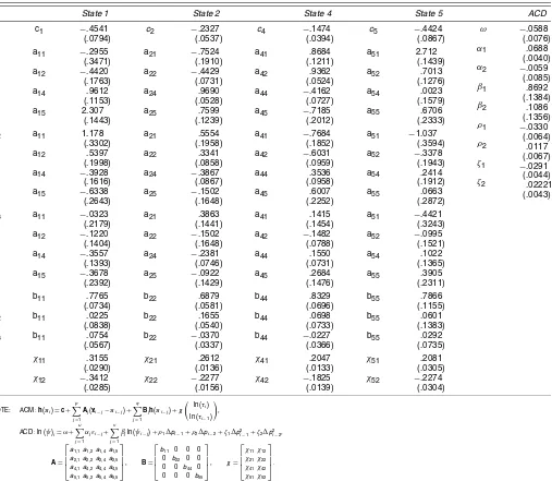
in favor of an ACM(3,3)–ACD(2,2)model with ap value is 6.7×10⁻⁵. The ACM(3,3)–ACD(2,2)model is not rejected for the ACM(4,4)–ACD(2,2) model with a p-value of .29, however. Further diagnostics suggest that no additional lags of the duration are needed in the ACM specification. Similarly, we also find that no additional price lags are needed in the ACD specification. Table 2 gives the parameter estimates for
Table 2. Parameter Estimates for the Unrestricted ACM(3, 3)–ACD(2, 2) Model
State 1 State 2 State 4 State 5 ACD
c1 −.4541 c2 −.2327 c4 −.1474 c5 −.4424 ω rors, of the estimates are given in parentheses.
Before discussing the parameter estimates, we examine the model diagnostics. As discussed in Section 3.2, the standard-ized residuals should be temporally uncorrelated. Figure 4 presents the correlations constructed for the standardized resid-uals given in (17). We again denote significant (at the 5% level) correlations, with a “+” or “−” indicating the sign. The strong correlations at lag 1 have vanished. Furthermore, the long sets of positive correlations in the raw series have also disappeared. A formal test for the null hypothesis that the standardized series is white noise can be obtained from the test statistic in (19). The
pvalue is .31, providing no evidence of remaining correlation. The one-step-ahead prediction errors, associated with each state are not correlated with past errors, indicating that the model is well specified.
Engle and Russell (1998) suggested using the standardized durations, given byei= τˆi
ψi, to assess the fit of the ACD model.
Under correct specification, this series should be distributed as
an iid unit exponential. The Ljung–Box test for the null hypoth-esis that the series is uncorrelated through the first 15 lags has apvalue of .11. The variance of the series indicates some re-maining excess dispersion, however.
4.3 Interpretation of Results and Hypothesis Tests
We now turn to interpretation of results. We begin by sum-marizing the parameter estimates and testing the symmetry con-ditions suggested in Section 3.3. Finally, we provide a detailed discussion of the nature of dependence between price changes and the durations implied by the model estimates. This relation-ship is related to market microstructure theories proposed in the literature.
The sum of thejth diagonal elements of theBi matrices of
an ACM model characterize the persistence associated with the
jth state. This persistence measure is similar across all states, with states 1 and 5 summing to .874 and .876 and states 2 and 4 summing to .803 and .88. The impact of the contemporaneous
Figure 4. Box–Tiao Representation of Sample Cross-Correlations of the Standardized Residual Vector.
and lagged durations on thejth price transition probabilities are given by χj1 andχj2. The coefficients on the contemporane-ous duration are positive and significant for all four states. Be-cause the log odds are taken with respect to the base state of no price change, this indicates that the probability of a price move increases with the duration. These estimates imply that the timing of transactions and the distribution of transaction-by-transaction price changes are related. We investigate this re-lationship later in this section.
Further examination of terms in the Aand B matrices re-veals structure. In particular, for eachAandBmatrix, row 5 is roughly the reverse, or mirror image, of row 1. Similarly, row 4 is roughly the reverse, or mirror image, of row 2. This is exactly what we would expect to find if the price symmetry hypothesis discussed in Section 3.3 were to hold. We now proceed to test several hypothesis of symmetry.
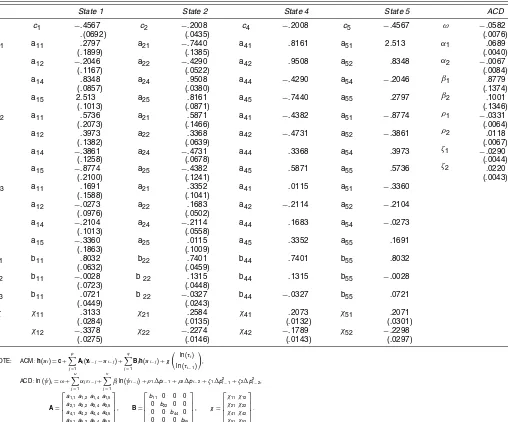
We first consider a test for dynamic price symmetry by jointly testing that the A and B matrices are all response-symmetric. The likelihood ratio test associated with the null hy-pothesis for theAandBmatrices is marginally not rejected at the 5% level with apvalue of .058. Hence we are unable to re-ject symmetry in the marginal impact of the past price changes on the future log odds. We are also unable to reject that the con-stant vectorcis symmetric. Thepvalue for this likelihood ratio test is .39. However, we strongly reject the null hypothesis that the coefficient vectors on the durationsχ1andχ2are symmet-ric vectors; thepvalue is 1.05×10⁻³. Table 3 gives the para-meter estimates for the price symmetric model with symmetric intercept but asymmetric duration impact.
The coefficients on the contemporaneous duration associated with the downward price moves are larger than those associated with upward price moves. Hence the probability of a downward price move increases more than the probability of an upward price move as the elapsed time since the last trade increases. Short elapsed time since the last transaction is associated with rising prices, and long elapsed time since the last transaction is associated with falling prices.
We now examine the relationship between the transaction price change and the elapsed time. Given the filtration of past price changes and durations, the variance of transaction price changes can be expressed conditionally as a function of the con-temporaneous duration. We plot the transaction price variance as a function ofτ, fixing the lagged values at their unconditional means and evaluating the conditional variance of price changes obtained by varying the contemporaneous duration. This plot is given in Figure 5. The variance is an upward-sloping func-tion of the contemporaneous durafunc-tion. For reference, each stan-dardized unit of time is, on average, a little over 3 minutes. It is interesting to compare the conditional variance to the vari-ance obtained when the log stock price follows a random walk. We calculate the variance of the open-to-close returns, then cal-culate the variance per unit of standardized time implied by Brownian motion. The upward-sloping line in Figure 5 is the Brownian motion variance as a function of the standardized time interval, which is linear in elapsed time. We convert from the variance of returns to variance of price changes by multi-plying by the square of the sample average price.
We might expect that the conditional transaction price vari-ance to be larger than the Brownian motion varivari-ance because the transaction price process includes both the variance of Brownian motion and market microstructure effects, such as price discreteness and other transitory effects. Even very short durations, may result in a price change equal to or greater than the minimum tick size. Indeed, for very short durations, the con-ditional variance from the ACM model is much higher than that implied by Brownian motion. What is interesting, however, is that the volatility is a concave function of the durationτ, with slope becoming smaller than that of the Brownian motion, so that the variance per unit time declines with duration. For short-duration trades, the variance is above that of the Brownian mo-tion volatility, and for long-duramo-tion trades it is below that of the Bownian motion volatility.
This analysis shows that for the Airgas stock, the timing of trades, and not merely the passage of time, affects volatility.
Table 3. Parameter Estimates for Restricted ACM(3, 3)–ACD(2, 2) Model
State 1 State 2 State 4 State 5 ACD
c1 −.4567 c2 −.2008 c4 −.2008 c5 −.4567 ω
This relationship is predicted by theoretical models where time-varying transaction rates are driven by discretionary-informed traders that trade only when they have superior information (for an early reference, see Easley and O’Hara 1992). In these mod-els, the price adjustments, and hence volatility, will be larger in periods of frequent trading and smaller when trades are infre-quent.
Figure 5 also presents a plot of the expected transaction price change given a durationτ and the filtration of past price changes obtained using the same method as for the variance. The conditional mean is a downward-sloping function of the time since the last trade. This result is in the same direction and much more significant than the mean effect noted by Engle (2000). The fact that long durations are associated with falling prices is consistent with the theoretical model of Diamond and Verrecchia (1987), who suggested that in the presence of short selling constraints, periods of infrequent trading are indicative of bad news. Agents who have bad news about the asset and would like to short the asset may be unable to do so, given short selling constraints.
Figure 5. Conditional Mean and Variance of Price Changes as a Function of Time Elapsed Since Previous Transaction ( mean;
variance; rw variance).
The coefficient on the lagged duration is negative for all states. For the two-tick price moves (states 1 and 5), the coef-ficient on the lagged duration is larger in magnitude than the coefficient on the contemporaneous duration. All else being equal, the net effect of a long duration beyond one period is to decrease the probability of a large price change. The coeffi-cient on the lagged duration is slightly smaller in magnitude for the one-tick price moves. The net effect of a long duration be-yond one period is to slightly lower the probability of a one-tick move. Long durations increase the probability of contempora-neous price moves but have a slight tendency to decrease the probability of price moves in expected multiple periods ahead.
Examining the coefficients associated with the ACD model, we find that lag-one coefficients of both the price change and its square are negative and significant, indicating that durations are expected to be shorter after upward price moves and/or larger price changes. This effect is partially offset by the lag-two co-efficients that are positive and significant for both the price changes and squared price changes.
5. CONCLUSIONS
In this article we have proposed modeling financial trans-actions data as a marked point process where the points are the transaction times and the associated marks are informa-tion about the transacinforma-tion, such as the price. Our approach in-volves decomposing the joint density of arrival times and price changes into the product of a conditional distribution for the price changes and a marginal distribution for the arrival times. Institutional features restrict prices to fall on discrete values. For our sample, the overwhelming majority of the price changes take one of just five different values. We therefore treated the price changes as a multinomial random variable and propose an autoregressive model for the price transition probabilities. We have examined some theoretical properties of our ACM model. We used the ACD model of Engle and Russell (1998) for the marginal distribution of the arrival times.
We found little evidence of time-of-day effects in the distrib-ution of transaction-by-transaction price for the stock analyzed. This has the interesting implication that the time-of-day pat-terns typically observed in within-day volatility measured over fixed time intervals is an artifact of the diurnal patterns in the transaction rate.
We estimated the joint ACM–ACD model by maximum like-lihood. A simple-to-general model selection approach suggests that moderately simple models appear to be adequate. This modeling approach provides a microscopic view of the intra-day dynamics of asset prices. For the NYSE stock analyzed, we tested for and found evidence of a type of symmetry in the mar-ginal impacts of the history of price changes on the transition probabilities.
We found that the transaction price variance increases with the duration but at a slower rate than would be implied by sim-ple geometric Brownian motion. In fact, the variance is virtually constant after a length of time equal to the mean duration has passed since the last transaction. This is consistent with pre-dictions from Easley and O’Hara (1992), where the absence of transactions is indicative of no private information in the market and slow adjustment of prices. Conversely, rapid transactions
are associated with the presence of informed trading so prices adjust quickly.
We also tested for and found that long durations are associ-ated with falling prices. This result is consistent with the theo-retical predictions of Diamond and Verrecchia (1987), in which short selling constraints suggest that long durations are indica-tive of “bad news.”
We believe that the ACM–ACD model may provide a use-ful tool for analyzing other discrete, potentially irregularly spaced data, such as credit risk dynamics or marketing data, where consumers face a discrete product choice set such as different brands. Recently, the NYSE and NASDQ completed its move to decimalization. It is also worth noting that for many stocks, the histogram of stock price changes measured in ticks looks remarkably similar in postdecimalization trans-actions data. Hence there is no reason to think that the model will not perform equally well on the current decimalized data. The ACD model may well provide a good approach to ana-lyzing how these changes affect the transaction costs (effective cost) or price dynamics.
Finally, we note that since the first draft of this article, nu-merous interesting alternative approaches to modeling discrete price changes have been proposed in the literature. Rydberg and Shephard (2000, 2003) have proposed an alternative model for discrete price movements, Bauwens and Giot (2003) have proposed an alternative competing risk model, and Prigent, Renault, and Scaillet (2001) have applied the two-state ACM model suggested here in an option pricing setting. Models that assume continuous distributions for returns have been consid-ered by Ghysels and Jasiak (1998) and Grammig and Wellner (2002).
ACKNOWLEDGMENTS
The authors are very grateful to the anonymous associate edi-tor who provided extensive suggestions. They also thank David Brillinger, Xiaohong Chen, Clive Granger, Jim Hamilton, Alex Kane, Bruce Lehman, Peter McCullagh, Glenn Sueyoshi, George Tiao, and Hal White for valuable input. The authors gratefully acknowledge financial support from the Sloan Foun-dation, the University of California, San Diego Project in Econometric Analysis, the University of Chicago Graduate School of Business, and the National Science Foundation (grant SBR-9422575).
APPENDIX A: SUMMARY OF SUPERSCRIPT/SUBSCRIPT NOTATION
For the random variable y, yi denotes the random variable
associated with transactioni, and
y(i−1)=(yi−1,yi−2, . . . ).
For a random vector w,wi denotes a vector associated with
transactioni, andwijdenotes thejth element of a vector
associ-ated with transactioni.
Unless otherwise specified, vectors with tildes have dimen-sionkand vectors without tildes have dimensionk−1.
For a matrixW,Wjdenotes thejth matrix, andWmndenotes
them,nelement.
For a constant vectorc,cmdenotes themth element.
APPENDIX B: PROOFS OF THEOREMS AND PROPOSITIONS
B.1 Proof of Theorem 1
The ACM(p,q) model with a vector of constants χ is
outside the unit circle, we can write
h(πi)=
Here||is an element-by-element absolute value. Next, note that the elements of|xi−πi|must lie between 0 and 1
inclu-sive, so it follows that
|h(πi)| ≤
on the probabilities are then obtained by setting
Mu=exp
where the exponential function is understood to be element by element. Because the probabilities are given by the logistic transformation, it follows that the elements ofπiare bounded
strictly away from 0,
πi≥
1
(ι′Mu+1)M
l>0. (B.5)
B.2 Proof of Proposition 1
Qh(πi.)= From the symmetry assumptions, it follows that
Qh(πi.)=
history generates the mirror-image log odds. Finally, recall that theith element ofhis simply the log(πi/π0), so it follows that
Qπi(xi−1,xi−2, . . . ,Zi)=πi(Qxi−1,Qxi−2, . . . ,Zi).
B.3 Proof of Proposition 2
We must show that thejof (2′) are response-symmetric,
(L)=
The last equality follows from the fact that the prices are dynamic-symmetric. Response-symmetricj then follows
im-mediately from the response symmetry of
[Received March 1998. Revised April 2004.]
REFERENCES
Ane, T., and Geman, H. (1999), “Stochastic Volatility and Transaction Time: An Activity Based Volatility Estimator,”The Journal of Risk, 2, 18. Bauwens, L., Galli, F., and Giot, P. (2002), “The Moments of Log-ACD
Mod-els,” CORE discussion paper.
Bauwens, L., and Giot, P. (2000), “The Logarithmic ACD Model: An Ap-plication to the Bid–Ask Quote Process of Three NYSE Stocks,”Annales d’Economie et de Statistique, 60, 117–149.
(2003), “Asymmetric ACD Models: Introducing Price Information in ACD Models With a Two-State Transition Model,”Empirical Economics, 28, 709–731.
Bauwens, L., Giot, P., Grammig, J., and Veredas, D. (2003), “A Comparison of Financial Duration Models via Density Forecasts,”International Journal of Forecasting, 20, 589–609.
Berndt, E., Hall, B., Hall, R., and Hausman, J. (1974), “Estimation and Infer-ence in Nonlinear Structural Models,”Annals of Economic and Social Mea-surement, 3, 653–665.
Cox, D. R. (1981), “Statistical Analysis of Time Series: Some Recent Develop-ments,”Scandinavian Journal of Statistics, 8, 93–115.
Diamond, D. W., and Verrecchia, R. E. (1987), “Constraints on Short-Selling and Asset Price Adjustments to Private Information,”Journal of Financial Economics, 18, 277–311.
Easley, D., and O’Hara, M. (1992), “Time and the Process of Security Price Adjustment,”The Journal of Finance, 19, 69–90.
Engle, R. (2000), “The Econometrics of Ultra-High Frequency Data,” Econo-metrica, 68, 1–22.
Engle, R., and Lunde, A. (2003), “Trades and Quotes: A Bivariate Point Process,”Journal of Financial Econometrics, 1, 159–188.
Engle, R., and Patton, A. (2003), “Impacts of Trades in an Error-Correction Model of Quote Prices,”Journal of Financial Markets, 7, 1–25.
Engle, R., and Russell, J. (1995), “Autoregressive Conditional Duration: A New Model for Irregularly Spaced Data,” unpublished manuscript, University of California, San Diego.
(1998), “Autoregressive Conditional Duration: A New Model for Ir-regularly Spaced Data,”Econometrica, 66, 1127–1162.
Ghysels, E., and Jasiak, J. (1998), “GARCH for Irregularly Spaced Data: The ACD–GARCH Model,”Studies in Nonlinear Economics and Econometrics, 2, 133–149.
Grammig, J., and Wellner, M. (2002), “Modeling the Interdependence of Volatility and Intertransaction Duration Processes,”Journal of Econometrics, 106, 369–400.
Harris, L. E. (1990) “Estimation of Stock Price Variance and Serial Covari-ances From Discrete Observations,”Journal of Financial and Quantitative Analysis, 25, 291–306.
Hasbrouck, J. (1991), “Measuring the Information Content of Stock Trades,”
Journal of Finance, 66, 179–207.
Hausman, J., Lo, A., and MacKinlay, C. (1992), “An Ordered Probit Analysis of Transaction Stock Prices,”Journal of Financial Economics, 31, 319–379. Jacobs, P., and Lewis, P. (1983), “Stationary Discrete Autoregressive-Moving Average Time Series Generated by Mixtures,”Journal of Time Series Analy-sis, 4, 19–36.
Jones, C., Kaul, G., and Lipson, M. (1994), “Transactions, Volume, and Volatil-ity,”Review of Financial Studies, 7, 631–651.
Kalbfleisch, J., and Prentice, R. (1980),The Statistical Analysis of Failure Time Data, New York: Wiley.
Lancaster, T. (1990),The Econometric Analysis of Transition Data, Cambridge, U.K.: Cambridge University Press.
Li, W. K., and McLeod, A. I. (1981), “Distribution of the Residual Autocorre-lations in Multivariate ARMA Time Series,”Journal of the Royal Statistical Society, Ser. B, 43, 231–239.
MacDonald, I., and Zucchini, W. (1997),Hidden Markov and Other Models for Discrete-Valued Time Series, New York: Chapman & Hall.
MacRae, E. (1977), “Estimation of Time-Varying Markov Processes With Ag-gregate Data,”Econometrica, 45, 183–198.
McInish, T., and Wood, R. (1992), “An Analysis of Intradaily Patterns in Bid/Ask Spreads for NYSE Stocks,”Journal of Finance, 47, 753–764. Nelson, D. (1991), “Conditional Heteroskedasticity in Asset Returns: A New
Approach,”Econometrica, 59, 347–370.
Prigent, J., Renault, E., and Scaillet, O. (2001), “An Autoregressive Conditional Binomial Option Pricing Model,” inSelected Papers From the First World Congress of the Bachelier Finance Society, New York: Springer-Verlag, pp. 353–374.
Rydberg, T., and Shephard, N. (2000), “A Modelling Framework for the Prices and Times Made on the New York Stock Exchange,” in Non-Stationary and Non-Linear Signal Extraction, eds. W. J. Fitzgerald, R. L. Smith, A. T. Walden, and P. C. Young, Cambridge, U.K.: Cambridge University Press, pp. 217–246.
(2003), “The Dynamics of Trade-by-Trade Price Movements,”Journal of Financial Econometrics, 1, 2–25.
Shephard, N. (1995), “Generalized Linear Autoregressions,” unpublished man-uscript, Nuffield College, Oxford.
Tiao, G., and Box, G. (1981), “Modeling Multiple Time Series With Applica-tions,”Journal of the American Statistical Association, 76, 802–816.