Understanding CPI dynamics in Canada

(1)

MPRA

Munich Personal RePEc Archive

Understanding CPI dynamics in Canada

THABANI NYONI

UNIVERSITY OF ZIMBABWE

15 February 2019

Online at

https://mpra.ub.uni-muenchen.de/92415/

(2)

Understanding CPI Dynamics in Canada Nyoni, Thabani Department of Economics University of Zimbabwe Harare, Zimbabwe Email: nyonithabani35@gmail.com ABSTRACT

This research uses annual time series data on CPI in Canada from 1960 to 2017, to model and forecast CPI using the Box – Jenkins ARIMA technique. Diagnostic tests indicate that the C series is I (1). The study presents the ARIMA (1, 1, 1) model for predicting CPI in Canada. The diagnostic tests further show that the presented parsimonious model is stable. The results of the study apparently show that CPI in Canada is likely to continue on a sharp upwards trajectory in the next decade. The study encourages policy makers to make use of tight monetary and fiscal policy measures in order to control inflation in Canada.

Key Words: Forecasting, Inflation

JEL Codes: C53, E31, E37, E47

INTRODUCTION

Inflation is one of the central terms in macroeconomics (Enke & Mehdiyev, 2014) as it harms the stability of the acquisition power of the national currency, affects economic growth because investment projects become riskier, distorts consuming and saving decisions, causes unequal income distribution and also results in difficulties in financial intervention (Hurtado et al, 2013). As the prediction of accurate inflation rates is a key component for setting the country’s monetary policy, it is especially important for central banks to obtain precise values (Mcnelis & Mcadam, 2004). Consumer Price Index (CPI) may be regarded as a summary statistic for frequency distribution of relative prices (Kharimah et al, 2015). CPI number measures changes in the general level of prices of a group of commodities. It thus measures changes in the purchasing power of money (Monga, 1977; Subhani & Panjwani, 2009). As it is a prominent reflector of inflationary trends in the economy, it is often treated as a litmus test of the

(3)

effectiveness of economic policies of the government of the day (Sarangi et al, 2018). The CPI program focuses on consumer expenditures on goods and services out of disposable income (Boskin et al, 1998). Hence, it excludes non-market activity, broader quality of life issues, and the costs and benefits of most government programs (Kharimah et al, 2015). To avoid adjusting policy and models by not using an inflation rate prediction can result in imprecise investment and saving decisions, potentially leading to economic instability (Enke & Mehdiyev, 2014). Precisely forecasting the change of CPI is significant to many aspects of economics, some examples include fiscal policy, financial markets and productivity. Also, building a stable and accurate model to forecast the CPI will have great significance for the public, policy makers and research scholars (Du et al, 2014). In this study we use CPI as an indicator of inflation in Canada and then attempt to model and forecast CPI in Canada using the Box-Jenkins ARIMA technique.

LITERATURE REVIEW

Zivko & Bosnjak (2017) studied inflation in Croatia using ARIMA models with a data set ranging over the period January 1997 to November 2015 and established that the ARIMA (0, 1, 1)x(0, 1, 1)12 is the optimal model for forecasting inflation in Croatia. In Albania, Dhamo et al

studied CPI using SARIMA models with a data set ranging over the period January 1994 to December 2007 and discovered that SARIMA models are satisfactory for a short-term prediction compared to the multiple regression model forecast. Nyoni (2018k) studied inflation in Zimbabwe using GARCH models with a data set ranging over the period July 2009 to July 2018 and established that there is evidence of volatility persistence for Zimbabwe’s monthly inflation data. Nyoni (2018n) modeled inflation in Kenya using ARIMA and GARCH models and relied on annual time series data over the period 1960 – 2017 and found out that the ARIMA (2, 2, 1) model, the ARIMA (1, 2, 0) model and the AR (1) – GARCH (1, 1) model are good models that can be used to forecast inflation in Kenya. Nyoni & Nathaniel (2019), based on ARMA, ARIMA and GARCH models; studied inflation in Nigeria using time series data on inflation rates from 1960 to 2016 and found out that the ARMA (1, 0, 2) model is the best model for forecasting inflation rates in Nigeria.

MATERIALS & METHODS Box – Jenkins ARIMA Models

One of the methods that are commonly used for forecasting time series data is the Autoregressive Integrated Moving Average (ARIMA) (Box & Jenkins, 1976; Brocwell & Davis, 2002; Chatfield, 2004; Wei, 2006; Cryer & Chan, 2008). For the purpose of forecasting Consumer Price Index (CPI) in Canada, ARIMA models were specified and estimated. If the sequence ∆dCt

satisfies an ARMA (p, q) process; then the sequence of Ct also satisfies the ARIMA (p, d, q)

process such that:

∆𝑑_𝐶 𝑡= ∑ 𝛽𝑖∆𝑑𝐶𝑡−𝑖+ 𝑝 𝑖=1 ∑ 𝛼𝑖𝜇𝑡−𝑖 𝑞 𝑖=1 + 𝜇𝑡… … … . … … … … . … … . [1]

(4)

∆𝑑_𝐶 𝑡 = ∑ 𝛽𝑖∆𝑑𝐿𝑖𝐶𝑡 𝑝 𝑖=1 + ∑ 𝛼𝑖𝐿𝑖𝜇𝑡 𝑞 𝑖=1 + 𝜇𝑡… … … . . … … … . … … … [2]

where ∆ is the difference operator, vector β ϵⱤp

and ɑ ϵⱤq.

The Box – Jenkins Methodology

The first step towards model selection is to difference the series in order to achieve stationarity. Once this process is over, the researcher will then examine the correlogram in order to decide on the appropriate orders of the AR and MA components. It is important to highlight the fact that this procedure (of choosing the AR and MA components) is biased towards the use of personal judgement because there are no clear – cut rules on how to decide on the appropriate AR and MA components. Therefore, experience plays a pivotal role in this regard. The next step is the estimation of the tentative model, after which diagnostic testing shall follow. Diagnostic checking is usually done by generating the set of residuals and testing whether they satisfy the characteristics of a white noise process. If not, there would be need for model re – specification and repetition of the same process; this time from the second stage. The process may go on and on until an appropriate model is identified (Nyoni, 2018i).

Data Collection

This study is based on a data set of annual CPI (C) in Canada ranging over the period 1960 – 2017. All the data was gathered from the World Bank.

Diagnostic Tests & Model Evaluation Stationarity Tests

The ADF Test

Table 1: Levels-intercept

Variable ADF Statistic Probability Critical Values Conclusion

C 0.089399 0.9622 -3.552666 @1% Non-stationary

-2.914517 @5% Non-stationary -2.595033 @10% Non-stationary Table 2: Levels-trend & intercept

C -2.236151 0.4608 -4.130526 @1% Non-stationary

-3.492149 @5% Non-stationary -3.174802 @10% Non-stationary Table 3: without intercept and trend & intercept

C 2.110425 0.9910 -2.606911 @1% Non-stationary

-1.946764 @5% Non-stationary -1.613062 @10% Non-stationary

(5)

Tables 1 – 3 indicate that C is non-stationary in levels.

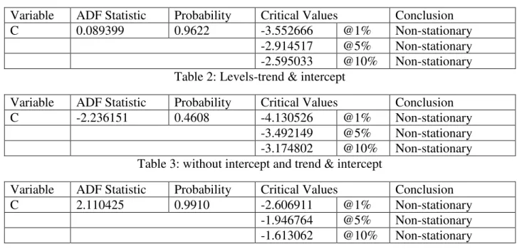
Table 4: 1st Difference-intercept

C -3.807637 0.0049 -3.552666 @1% Stationary

-2.914517 @5% Stationary -2.595033 @10% Stationary Table 5: 1st Difference-trend & intercept

C -3.775706 0.0253 -4.130526 @1% Non-stationary

-3.492149 @5% Stationary -3.174802 @10% Stationary Table 6: 1st Difference-without intercept and trend & intercept

C -10.15676 0.0000 -3.555023 @1% Stationary

-2.915522 @5% Stationary -2.595565 @10% Stationary Tables 4 – 6 indicate that the C series is stationary after taking first differences.

Evaluation of ARIMA models (with a constant)

Table 7

Model AIC U ME MAE RMSE MAPE

ARIMA (1, 1, 1) 153.9987 0.48666 0.033196 0.67787 0.87766 1.8374 ARIMA (1, 1, 0) 154.07 0.52295 0.018302 0.67913 0.89392 1.9378 ARIMA (0, 1, 1) 163.8655 0.66239 0.0072621 0.74061 0.96917 2.2244 ARIMA (2, 1, 1) 155.8095 0.48723 0.03899 0.68168 0.87611 1.8464 ARIMA (1, 1, 2) 155.7938 0.48765 0.039006 0.68152 0.87601 1.8478 ARIMA (2, 1, 2) 157.7934 0.48763 0.033909 0.68161 0.876 1.8479 A model with a lower AIC value is better than the one with a higher AIC value (Nyoni, 2018n). Theil’s U must lie between 0 and 1, of which the closer it is to 0, the better the forecast method (Nyoni, 2018l). The study will consider both the AIC and the U as the criterion for choosing the best model for forecasting CPI in Canada. Therefore, the ARIMA (1, 1, 1) model is eventually selected.

Residual & Stability Tests

ADF Tests of the Residuals of the ARIMA (1, 1, 1) Model

Table 8: Levels-intercept

Rt -7.015789 0.0000 -3.555023 @1% Stationary

(6)

-2.595565 @10% Stationary Table 9: Levels-trend & intercept

Rt -6.943109 0.0000 -4.133838 @1% Stationary

-3.493692 @5% Stationary -3.175693 @10% Stationary Table 10: without intercept and trend & intercept

Rt -7.080735 0.0000 -2.607686 @1% Stationary

-1.946878 @5% Stationary -1.612999 @10% Stationary Tables 8, 9 and 10 reveal that the residuals of the ARIMA (1, 1, 1) model are stationary.

Stability Test of the ARIMA (1, 1, 1) Model

Figure 1

Since the corresponding inverse roots of the characteristic polynomial lie in the unit circle, it illustrates that the chosen ARIMA (1, 1, 1) model is indeed stable and suitable for predicting CPI in Canada over the period under study.

FINDINGS Descriptive Statistics Table 11 -1.5 -1.0 -0.5 0.0 0.5 1.0 1.5 -1.5 -1.0 -0.5 0.0 0.5 1.0 1.5 AR roots MA roots

(7)

Description Statistic Mean 58.862 Median 62.5 Minimum 13 Maximum 112 Standard deviation 33.528 Skewness -0.032287 Excess kurtosis -1.4415

As shown above, the mean is positive, i.e. 58.862. The minimum is 13 while the maximum is 112. The skewness is -0.032287 and the most striking characteristic is that it is positive, indicating that the C series is positively skewed and non-symmetric. Excess kurtosis is -1.4415; showing that the C series is not normally distributed.

Results Presentation1 Table 12 ARIMA (1, 1, 1) Model: ∆𝐶𝑡−1= 1.64731 + 0.816188∆𝐶𝑡−1− 0.342036𝜇𝑡−1… … … . [3] P: (0.0000) (0.0000) (0.0704) S. E: (0.3709) (0.1138) (0.1891)

Variable Coefficient Standard Error z p-value

Constant 1.64731 0.370874 4.442 0.0000***

AR (1) 0.816188 0.11383 7.17 0.0000***

MA (1) -0.342036 0.189055 -1.809 0.0704*

The model constant is positive and statistically significant at 1% level of significance. This points to the fact that CPI in Canada cannot go below 1.65 even if the effect of the MA and AR components were to be ruled out. The coefficient of the AR (1) component is positive and statistically significant at 1% level of significance. This basically points to the fact that previous period CPI indices are important in determining the current and future levels of CPI in Canada. For example, when previous period CPI was relatively high; it arguably causes economic agents to anticipate even higher inflationary pressures in the next period thereby inducing policy ineffectiveness: in the long-run inflation goes up. The results of the study indicate that a 1% increase in the previous period CPI will lead to approximately 0.8% increase in the current period CPI. The coefficient of the MA (1) component is negative and statistically significant at 10% level of significance. This implies that unobserved shocks to CPI have a negative effect on current CPI in Canada. Such shocks include but are not limited to monetary policy shocks and political events. The results actually show that a 1% increase in such shocks will lead to approximately 0.34% decrease in CPI, thus a reduced level of inflation. For example, if a new government or political dispensation is elected into power in Canada; it could lower inflationary expectations and thereby enable policy makers to smoothly engineer disinflation and hence lower

1

(8)

CPI levels. The overall striking feature of these results is that the coefficient of the AR (1) component is positive while the coefficient of the MA (1) component is negative as conventionally expected.

Forecast Graph

Figure 2

Predicted CPI in Canada

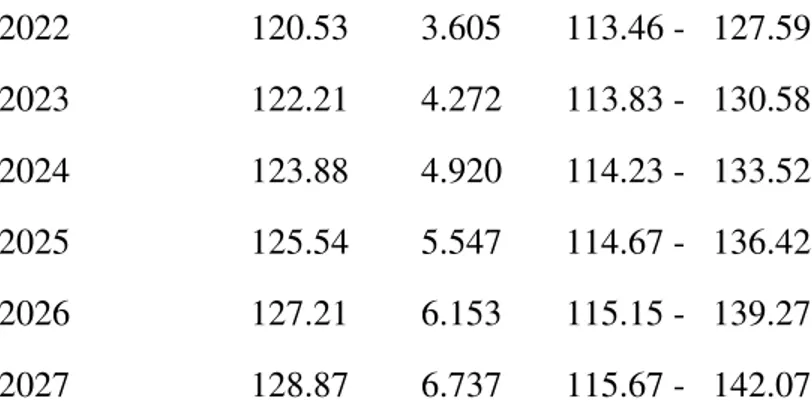
Table 13

Year Prediction Std. Error 95% Confidence Interval 2018 113.73 0.867 112.03 - 115.43 2019 115.45 1.544 112.42 - 118.47 2020 117.15 2.232 112.77 - 121.53 2021 118.84 2.923 113.11 - 124.57 0 20 40 60 80 100 120 140 160 1970 1980 1990 2000 2010 2020 95 percent interval CPI forecast

(9)

2022 120.53 3.605 113.46 - 127.59 2023 122.21 4.272 113.83 - 130.58 2024 123.88 4.920 114.23 - 133.52 2025 125.54 5.547 114.67 - 136.42 2026 127.21 6.153 115.15 - 139.27 2027 128.87 6.737 115.67 - 142.07

Figure 2 (with a forecast range from 2018 – 2027) and table 13, clearly show that CPI in Canada is indeed set to continue rising sharply, in the next decade.

POLICY IMPLICATION & CONCLUSION

After performing the Box-Jenkins approach, the ARIMA was engaged to investigate annual CPI of Canada from 1960 to 2017. The study mostly planned to forecast the annual CPI in Canada for the upcoming period from 2018 to 2027 and the best fitting model was selected based on how well the model captures the stochastic variation in the data. The ARIMA (1, 1, 1) model, as indicated by the AIC statistic; is not only stable but also the most suitable model to forecast the CPI of Canada for the next ten years. In general, CPI in Canada; showed an upwards trend over the forecasted period. Based on the results, policy makers in Canada should engage more proper economic and monetary policies in order to fight such increase in inflation as reflected in the forecasts. Therefore, relevant authorities in Canada ought to rely more on tight monetary policy, which should be complimented by a tight fiscal policy stance.

REFERENCES

[1] Boskin, M. J., Ellen, R. D., Gordon, R. J., Grilliches, Z & Jorgenson, D. W (1998). Consumer Price Index and the Cost of Living, The Journal of Economic Perspectives, 12 (1): 3 – 26.

[2] Box, G. E. P & Jenkins, G. M (1976). Time Series Analysis: Forecasting and Control,

Holden Day, San Francisco.

[3] Brocwell, P. J & Davis, R. A (2002). Introduction to Time Series and Forecasting,

Springer, New York.

[4] Chatfield, C (2004). The Analysis of Time Series: An Introduction, 6th Edition, Chapman & Hall, New York.

[5] Cryer, J. D & Chan, K. S (2008). Time Series Analysis with Application in R, Springer, New York.

[6] Dhamo, E., Puka, L & Zacaj, O (2018). Forecasting Consumer Price Index (CPI) using time series models and multi-regression models (Albania Case Study), Financial Engineering, pp: 1 – 8.

(10)

[7] Du, Y., Cai, Y., Chen, M., Xu, W., Yuan, H & Li, T (2014). A novel divide-and-conquer model for CPI prediction using ARIMA, Gray Model and BPNN, Procedia Computer Science, 31 (2014): 842 – 851.

[8] Enke, D & Mehdiyev, N (2014). A Hybrid Neuro-Fuzzy Model to Forecast Inflation,

Procedia Computer Science, 36 (2014): 254 – 260.

[9] Hurtado, C., Luis, J., Fregoso, C & Hector, J (2013). Forecasting Mexican Inflation Using Neural Networks, International Conference on Electronics, Communications and Computing, 2013: 32 – 35.

[10] Kharimah, F., Usman, M., Elfaki, W & Elfaki, F. A. M (2015). Time Series Modelling and Forecasting of the Consumer Price Bandar Lampung, Sci. Int (Lahore)., 27 (5): 4119 – 4624.

[11] Manga, G. S (1977). Mathematics and Statistics for Economics, Vikas Publishing House, New Delhi.

[12] Mcnelis, P. D & Mcadam, P (2004). Forecasting Inflation with Think Models and Neural Networks, Working Paper Series, European Central Bank.

[13] Nyoni, T & Nathaniel, S. P (2019). Modeling Rates of Inflation in Nigeria: An Application of ARMA, ARIMA and GARCH models, Munich University Library – Munich Personal RePEc Archive (MPRA), Paper No. 91351.

[14] Nyoni, T (2018k). Modeling and Forecasting Inflation in Zimbabwe: a Generalized Autoregressive Conditionally Heteroskedastic (GARCH) approach, Munich University Library – Munich Personal RePEc Archive (MPRA), Paper No. 88132.

[15] Nyoni, T (2018l). Modeling Forecasting Naira / USD Exchange Rate in Nigeria: a Box – Jenkins ARIMA approach, University of Munich Library – Munich Personal RePEc Archive (MPRA), Paper No. 88622.

[16] Nyoni, T (2018n). Modeling and Forecasting Inflation in Kenya: Recent Insights from ARIMA and GARCH analysis, Dimorian Review, 5 (6): 16 – 40.

[17] Nyoni, T. (2018i). Box – Jenkins ARIMA Approach to Predicting net FDI inflows in Zimbabwe, Munich University Library – Munich Personal RePEc Archive (MPRA), Paper No. 87737.

[18] Sarangi, P. K., Sinha, D., Sinha, S & Sharma, M (2018). Forecasting Consumer Price Index using Neural Networks models, Innovative Practices in Operations Management and Information Technology – Apeejay School of Management, pp: 84 – 93.

(11)

[19] Subhani, M. I & Panjwani, K (2009). Relationship between Consumer Price Index (CPI) and Government Bonds, South Asian Journal of Management Sciences, 3 (1): 11 – 17.

[20] Wei, W. S (2006). Time Series Analysis: Univariate and Multivariate Methods, 2nd Edition, Pearson Education Inc, Canada.

[21] Zivko, I & Bosnjak, M (2017). Time series modeling of inflation and its volatility in Croatia, Journal of Sustainable Development, pp: 1 – 10.