Learning to Program with MATLAB

(1)

(2)

(3)

LEARNING TO PROGRAM

WITH MATLAB

Building GUI Tools

(4)

ASSOCIATE PUBLISHER: Dan Sayre EDITORIAL ASSISTANT: Jessica Knecht MARKETING MANAGER: Christopher Ruel

DESIGNER: Kenji Ngieng

SENIOR PRODUCTION MANAGER: Janis Soo ASSOCIATE PRODUCTION MANAGER: Joyce Poh

This book was set by MPS Limited, Chennai. Cover and text printed and bound by Courier Westford.

This book is printed on acid free paper.

Founded in 1807, John Wiley & Sons, Inc. has been a valued source of knowledge and understanding for more than 200 years, helping people around the world meet their needs and fulﬁll their aspirations. Our company is built on a foundation of principles that include responsibility to the communities we serve and where we live and work. In 2008, we launched a Corporate Citizenship Initiative, a global effort to address the environmental, social, economic, and ethical challenges we face in our business. Among the issues we are addressing are carbon impact, paper speciﬁcations and procurement, ethical conduct within our business and among our vendors, and community and charitable support. For more information, please visit our website:

www.wiley.com/go/citizenship.

Copyright © 2013 John Wiley & Sons, Inc. All rights reserved. No part of this publication may be reproduced, stored in a retrieval system or transmitted in any form or by any means, electronic, mechanical, photocopying, recording, scanning or otherwise, except as permitted under Sections 107 or 108 of the 1976 United States Copyright Act, without either the prior written permission of the Publisher, or authorization through payment of the appropriate per-copy fee to the Copyright Clearance Center, Inc. 222 Rosewood Drive, Danvers, MA 01923, website www.copyright.com. Requests to the Publisher for permission should be addressed to the Permissions Department, John Wiley & Sons, Inc., 111 River Street, Hoboken, NJ 07030-5774, (201)748-6011, fax (201)748-6008, website http://www.wiley.com/go/permissions.

Evaluation copies are provided to qualiﬁed academics and professionals for review purposes only, for use in their courses during the next academic year. These copies are licensed and may not be sold or transferred to a third party. Upon completion of the review period, please return the evaluation copy to Wiley. Return instructions and a free of charge return mailing label are available at www.wiley.com/go/returnlabel. If you have chosen to adopt this textbook for use in your course, please accept this book as your complimentary desk copy. Outside of the United States, please contact your local sales representative.

Library of Congress Cataloging-in-Publication Data Lent, Craig S., 1956–

Learning to program with MATLAB : building GUI tools / Craig S. Lent, Department of Electrical Engineering, University of Notre Dame.

pages cm Includes index.

ISBN 978-0-470-93644-3 (pbk. : acid-free paper) 1. Computer programming.

2. Visual programming (Computer science) 3. MATLAB. 4. Graphical user interfaces (Computer systems) I. Title.

QA76.6.L45 2013 005.4'37—dc23

2012041638

Printed in the United States of America

(5)

(6)

(7)

Preface

To learn how to program a computer in a modern language with serious graphical capa-bilities, is to take hold of a tool of remarkable flexibility that has the power to provide profound insight. This text is primarily aimed at being a first course in programming, and is oriented toward integration with science, mathematics, and engineering. It is also use-ful for more advanced students and researchers who want to rapidly acquire the ability to easily build useful graphical tools for exploring computational models. The MATLAB programming language provides an excellent introductory language, with built-in graph-ical, mathematgraph-ical, and user-interface capabilities. The goal is that the student learns to build computational models with graphical user interfaces (GUIs) that enable exploration of model behavior. This GUI tool-building approach has been used at multiple educational levels: graduate courses, intermediate undergraduate courses, an introductory engineering course for first-year college students, and high school junior and senior-level courses.

The MATLAB programming language, descended from FORTRAN, has evolved to include many powerful and convenient graphical and analysis tools. It has become an important platform for engineering and science education, as well as research. MATLAB is a very valuable ﬁrst programming language, and for many will be the preferred language for most, if not all, of the computational work they do. Of course, C₊₊, Java, Python, and many other languages play crucial roles in other domains. Several language features make the MATLAB language easier for beginners than many alternatives: it is interpreted rather than compiled; variable types and array sizes need not be declared in advance; it is not strongly typed; vector, matrix, multidimensional array, and complex numbers are basic data types; there is a sophisticated integrated development and debugging environment; and a rich set of mathematical and graphics functions is provided.

While computer programs can be used in many ways, the emphasis here is on building computational models, primarily of physical phenomena (though the techniques can be easily extended to other systems). A physical system is modeled first conceptually, using ideas such as momentum, force, energy, reactions, fields, etc. These concepts are expressed mathematically and applied to a particular class of problem. Such a class might be, for example, projectile motion, fluid flow, quantum evolution, electromagnetic fields, circuit equations, or Newton’s laws. Typically, the model involves a set of parameters that describe the physical system and a set of mathematical relations (systems of equations, integrals, differential equations, eigensystems, etc.). The mathematical solution process must be realized through a computational algorithm—a step-by-step procedure for calculating the desired quantities from the input parameters. The behavior of the model is then usually visualized graphically, e.g., one or more plots, bar graphs, or animations.

(12)

A GUI tool consists of a computational model and a graphical user interface that lets the user easily and naturally adjust the parameters of the model, rerun the computation, and see the new results.

The experience that led to this text was the observation that student learning is enhanced if the students themselves build the GUI tool: construct the computational model, implement the visualization of results, and design the GUI.

The GUI is valuable for several reasons. The most important is that exploring model behav-ior, by manipulating sliders, buttons, checkboxes, and the like, encourages a focus on developing an intuitive insight into the model behavior. Insight is the primary goal. Run-ning the model many times with differing inputs, the user can start to see the characteristic behavior of physical system represented by the model. Additionally, it must be recognized that graphically driven tools are what students are accustomed to when dealing with com-puters. A command line interface seems crude and retrograde. Moreover, particularly for engineering students, the discipline of wrapping the model in a form that someoneelsecould use encourages a design-oriented mentality. Finally, building and delivering a sophisticated mathematical model that is operated through a GUI interface is simply more rewarding and fun.

The GUI tool orientation guides the structure of the text. Part I (Chapters 1 through 8) covers the fundamentals of MATLAB programming and basic graphics. It is designed to be what one needs to know prior to actual GUI building. The goal is to get the student ready for GUI building as quickly as possible (but not quicker).

In this context, Chapter 4 (matrices) and Chapter 6 (animation) warrant comment. Because arrays are a basic MATLAB data class and solving linear systems a frequent application, this material is included in Part I. An instructor could choose to cover it later without disrupting the ﬂow of the course. Similarly, the animation techniques covered in Chapter 6 could be deferred. The animation process does, however, provide very helpful and enjoyable practice at programming FOR loops. Many GUI tools are enhanced by having an animation compo-nent; among other advantages, animation provides a ﬁrst check of model behavior against experience. The end of Chapter 6 also includes a detailed discussion of the velocity Verlet algorithm as an improvement on the Euler method for solving systems governed by Newton’s second law. While this could be considered a more advanced topic, without it, models as sim-ple as harmonic motion or bouncing balls fail badly because of nonconservation of energy.

Part II covers GUI tool creation with the GUIDE (graphical user interface development environment) program, which is part of MATLAB. Chapters 9 and 10 are the heart of the text and take a very tutorial approach to GUI building. Chapter 10 details a simple, but widely useful, technique for transforming a functioning MATLAB program into a GUI tool. Readers already familiar with MATLAB, but unfamiliar with using GUIDE, can likely work through these two chapter in a couple hours and be in short order making GUI tools.

(13)

simplest way to invoke a particular function; more complicated uses are left for the student to explore using the documentation.

This approach—having students write GUI tools for speciﬁc problem domains—grew out of the author’s experience teaching undergraduate electromagnetics courses and graduate quantum mechanics courses in electrical engineering at the University of Notre Dame. These areas are characterized by a high level of mathematical abstraction, so having students transform the esoteric mathematics ﬁrst into code, and then into visualizable answers, proved invaluable.

The text began as a set of lecture notes for high school students at Trinity School at Green-lawn, in South Bend, Indiana. Since 2005, all Trinity juniors have learned MATLAB using this approach and have used it extensively in the physics and calculus courses that span the junior and senior year. The two other Trinity School campuses, one in Falls Church, Vir-ginia, and the other in Eagan, Minnesota, adopted the curriculum soon after the Greenlawn campus. The last chapter on mathematics is largely shaped by the material covered in the Trinity senior year. The author is profoundly grateful to the faculty and students of Trinity Schools, for their feedback, love of learning, and courage. Special thanks to Tom Finke, the remarkable head of Math and Science for Trinity Schools, and to Dr. John Vogel of Trinity School at Meadow View, for very helpful reviews of the manuscript. All author’s royalties from this text will go to support Trinity Schools. I’m very grateful to Tom Noe and Linda DeCelles for their help in preparing the manuscipt.

Since 2010, this approach to learning MATLAB, and the earlier preprints of the text, has been used in the Introduction to Engineering course for ﬁrst-year students in the College of Engineering at Notre Dame. In addition to learning to make MATLAB GUI tools, students employ them as part of a semester project completed in small teams. Each project nor-mally has a substantial physical apparatus (involving signiﬁcant construction), as well as an associated computational model. Some of the more specialized graphics topics included in Part III have been selected because they tend to arise in these projects. The course includes several other modules in addition to MATLAB and is the creation of Prof. Jay Brockman, a masterful teacher with profound pedagogical insights.

It is worth noting that in both the ﬁrst-year college engineering and high school contexts, students beneﬁt from a brief experience with a simpler programming language. At Notre Dame, this simpler language is the Lego robotics ROBOLAB®language for programming Lego Mindstorms®_{robots. The high school curriculum at Trinity introduces students to} pro-gramming with a four-week course on the Alice language, developed by Carnegie Mellon University. These “ramp languages” allow students to become accustomed to programming as creating a sequence of instructions in a way that is insulated from syntax errors.

A note on formatting: Numerous examples, programs, and code fragments are included in highlighted text. When the example is meant to illustrate the behavior of MATLAB commands typed in the Command window, the MATLAB command prompt “>>” is included, as in

(14)

Program listings, by contrast, contain the code as it would be seen in the Editor window.

%% greetings.m

% Greet user in cheery way % Author: Calvin Manthorn greeting='Hello, world!'; disp(greeting);

(15)

MATLAB Programming

(16)

(17)

Getting Started

1

1.1 Running the MATLAB IDE

1.2 MATLAB variables

1.3 Numbers and functions

1.4 Documentation

1.5 Writing simple MATLAB scripts

1.6 A few words about errors and debugging

1.7 Using the debugger

This chapter will introduce the basics of using MATLAB, ﬁrst as a powerful calculator, and then as a platform for writing simple programs that automate what a calculator would do in many steps. The emphasis here will be on performing basic mathematical operations on numbers.

The MATLAB integrated development environment is the program that runs when you launch MATLAB. You will use it to operate MATLAB interactively, and to develop and run MATLAB programs.

The concept of a MATLAB variable is important to grasp. It is not identical with the familiar mathematical notion of a variable, though the two are related. MATLAB variables should be thought of as labeled boxes that hold a number, or other type of information.

MATLAB has many built-in functions for evaluating common mathematical functions. More complicated MATLAB functions, including those of your own making, will be explored further in Chapter 7.

After completing this chapter you should be able to:

• Use the MATLAB integrated development environment to operate MATLAB interac-tively from within the Command window.

• Create and name MATLAB variables, and assign them numerical values.

• Invoke several built-in MATLAB mathematical functions (like sine, cosine, and exponential functions).

• Get more information on MATLAB statements and functions using thehelpanddoc

commands.

• Write a simple program that sets the values of variables, calculates some quantities, and then displays the results in the Command window.

• Run through a program line by line using the MATLAB debugger in the Editor window.

(18)

1.1 _{Running the MATLAB IDE}

MATLAB is normally operated from within the MATLAB integrated development envi-ronment (IDE). You can launch MATLAB in the Windows envienvi-ronment by double-clicking on the shortcut on your desktop, or by selecting it from the Start_|Programs menu.

The IDE is organized into a header menu bar and several different windows. Which windows are displayed can be determined by checking or unchecking items under the Layout menu on the HOME tab. Some important windows for working with MATLAB are:

Command window. This is the main interactive interface to MATLAB. To issue a MATLAB command, type the command at the>>prompt and press Enter on the keyboard. Workspace browser. Each variable deﬁned in the current workspace is represented here.

The name, class (type), value, and other properties of the variable can be shown. Choose which properties to show using the View—Choose Columns menu from the header menu bar. A recommended set to display is: Name, Value, and Class. Double-clicking on a variable brings up the Variable Editor window. The icon representing numbers is meant to symbolize an array, i.e., a vector or matrix. MATLAB’s basic data type is the array— a number is treated as a 1_×1 array.

Current Folder browser. In Windows parlance, the current folder is the same as the current directory. Without further instruction, MATLAB will save files in the current folder and look for files in the current directory. The browser displays files and other directories (folders) that reside in the current directory. Icons at the top of the browser allow the user to move up a directory (folder) level or to create a new folder. Double-clicking on a displayed folder makes it the current folder.

Editor window. The MATLAB editor is where programs are written. Launch the Editor window by typing “edit” in the Command window and pressing Enter. It doubles as part of the debugger interface, which is covered in detail later. The editor “knows” the MATLAB language and color codes language elements. There are many other convenient features to aid code-writing.

Figures window. Graphics is one of the main tools for visualizing numerical quantities. The results of executing graphics-related commands, such as those for plotting lines and surfaces, are displayed in the Figures window.

Variable Editor. The value or values held in a particular variable are displayed in a spreadsheet-like tool. This is particularly useful for arrays (matrices and vectors).

Manipulating windows

(19)

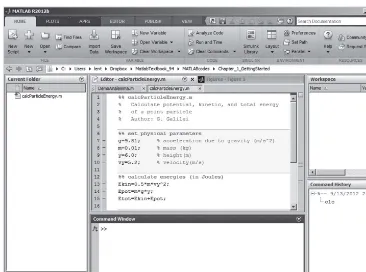
F I G U R E 1.1 The MATLAB integrated development environment (IDE) with the default layout.

Windows can be manipulated within the IDE by clicking and dragging the top frame of the window. Outlines of the drop position of the window appear and disappear as the mouse is moved around. This takes some practice.

More than one IDE window can share the same screen pane. Choose between active windows in a single pane by using the tabs at the top, side, or bottom of the of the pane.

The default window layout in the IDE is shown in Figure 1.1. A (strongly) recommended setup for the desktop includes three panel areas, as shown in Figure 1.2. In the upper left quadrant of the IDE position the Workspace browser, Current Folder browser, and (option-ally) the Figures window. One of these three is visible at any time, with the others being accessible by clicking the labeled tab. In the lower left, have the Command window open. The right portion is then devoted to the Editor window, where most of your program-ming work will take place. It really helps the development process to adopt this setup, or something very like it.

1.2 _{MATLAB variables}

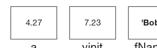
A MATLAB variable is simply a place in the computer’s memory that can hold information. Each variable has a speciﬁc address in the computer’s memory. The address is not manip-ulated directly by a MATLAB program. Rather, each variable is associated with a name that is used to refer to its contents. Each variable has aname, such asx,initialVelocity, or

(20)

Command Window tab-selected

Editor Window Figures

Current Folder

Workspace

F I G U R E 1.2 Recommended layout of the MATLAB IDE windows.

actually stored in the variable. The value may be a structured set of information, such as a matrix or a string of characters.

(21)

4.27 7.23

a

vinit

fName

'Bob'

F I G U R E 1.3 A schematic representation of MATLAB variablesa,vinit, andfName. Each has a name, class (type), and a current value.

the valuetrueorfalse, are stored in variables of thelogicalclass. Logical true and false are represented by a 1 and a 0. Other variable classes will be discussed later.

Variable assignment statements

The equals sign is the MATLAB assignment statement. The commanda=5stores the value 5 in the variable nameda. If the variableahas not already been created, this command will create it, then store the value. The class of the variable (its type) is determined by the value that is to be stored. Assignment statements can be typed into the Command window at the command prompt, a double greater-than symbol, “>>”.

>> a=4; % class double >> fname='Robert'; % class char >> temperature=101.2; % class double >> isDone=true; % class logical

In these examples, everything after the percent sign is a comment, information useful to the reader but ignored by MATLAB.

The assignment statement will cause MATLAB to echo the assignment to the Command window unless it is terminated by a semicolon.

>> a=4.2 a =

4.2000 >> a=5.5; >>

Multiple commands can be put on one line if they are separated by semicolons, though this is generally to be avoided because it degrades readability. We will occasionally do this in the text for brevity.

The right-hand side of the assignment statement can be anexpression, i.e., a combination of numbers, arithmetic operators, and functions.

>> a=4*7+2.2; >> r=a+b; >> b=sin(3.28);

>> x2=x1+4*sin(theta);

(22)

The general form of the assignment statement is

<variable name>=<expression>;

The expression is ﬁrst evaluated, then the value is stored in the variable named on the left-hand side of the equals sign. If variables appear in the expression on the right-hand side of the equals sign, the expression is evaluated by replacing the variable names in the expression with the values of the variablesat the time the statement is executed.Note that this does not establish an ongoing relationship between those variables.

>> a=5; >> b=7;

>> c=a+b % uses current values of a and b c =

12 >> a=0; >> b=-2; >> c c =

12 % kept same value despite a and b changing

The equals sign is used to store a result in a particular variable. The only thing permitted to the left of the equals sign is the variable name for which the assignment is to be made. Though the statementa=4looks like a mathematical equality, it is in factnota mathematical equation. None of the following expressions are valid:

>> r=a=4; % not a valid MATLAB statement >> a+1=press-2; % not a valid MATLAB statement >> 4=a; % not a valid MATLAB statement >> 'only the lonely'='how I feel'; % not a valid MATLAB

statement

By contrast this, which makes no sense as mathematics, is quite valid:

>> nr=nr+1; % increment nr

Variable names

(23)

chances for misspellings, which might go undetected. Only the ﬁrst 31 characters of the variable name are signiﬁcant.

xinit okay

VRightInitial okay

4You2do not okay

Start-up not okay

vector%1 not okay

TargetOne okay

ThisIsAVeryVeryLongVariableName okay

ThisIsAVeryVeryLongVariablename okay, but different from previous

x_temp okay

Variable workspace

The currently deﬁned variables exist in the MATLAB workspace. [We will see later that it’s possible for different parts of a program (separate functions) to have their own separate workspaces; for now there’s just one workspace.] The workspace is part of the dynamic memory of the computer. Items in the workspace will vanish when the current MATLAB session is ended (i.e., when we quit MATLAB). The workspace can be saved to a ﬁle and reloaded later, although use of this feature will be rare. The workspace can be managed further using the following commands:

clear a v g clears the variablesa v gfrom the workspace

clear clears all variables from the workspace

who lists the currently deﬁned variables

whos displays a detailed list of deﬁned variables

save saves the current workspace to the ﬁle called matlab.mat

save foobar saves the current workspace to the ﬁle called foobar.mat

load loads variables saved in matlab.mat into the current workspace

load foobar loads variables saved in foobar.mat into the current workspace

1.3 _{Numbers and functions}

While real numbers (class double) are precise to about 16 digits, the display defaults to showing fewer digits. The commandformat longmakes the display show more digits. The commandformat short, or justformat, resets the display.

Large numbers and small numbers can be entered using scientiﬁc notation. The number 6.0221415_×1023_{can be entered as}_6.0221415e23_{. The number}₋₁_.₆₀₂_×₁₀−19_{can be} entered as-1.602e-19.

(24)

recognizes the namepias the value 3.141592653589793. This can also be overwritten by deﬁning a variable namedpi, an extraordinarily bad idea.

Internally MATLAB represents real numbers in normalized exponential base-2 notation. The range of numbers is roughly from as small as 10−308_{to as large as 10}308_.

Standard numerical operations are denoted by the usual symbols, and a very large number of functions are available. Some examples follow.

+ addition

- subtraction

* multiplication

/ division

ˆ exponentiation, e.g., 1.3ˆ3.2 is 1.33.2

sin(x) returns the sine ofx

sind(x) returns the sine ofxdegrees

cos(x) returns the cosine ofx

cosd(x) returns the cosine ofxdegrees

tan(x) returns the tangent ofx

tand(x) returns the tangent ofxdegrees

atan(x) returns the inverse tangent ofx

atand(x) returns the inverse tangent ofxin degrees

acos(x) returns the inverse cosine ofx

acosd(x) returns the inverse cosine ofxin degrees

asin(x) returns the inverse sine ofx

asind(x) returns the inverse sind ofxin degrees

exp(x) returnsex

log(x) returns the natural logarithm ofx

log10(x) returns the log10(x)

sqrt(x) returns the square root ofx

abs(x) returns the absolute value ofx

round(x) returns the integer closest tox

ceil(x) returns the smallest integer greater than or equal tox

floor(x) returns the largest integer less than or equal tox

isprime(n) returns true ifnis prime

factor(k) returns prime factors ofk

sign(x) returns the sign (1 or₋1) ofx;sign(0)is 0

rand returns a pseudorandom number between 0 and 1

rand(m) returns anm_×marray of random numbers

rand(m,n) returns anm_×narray of random numbers

(25)

1.4 _{Documentation}

There are many MATLAB commands and functions. To get more information on a partic-ular command, including syntax and examples, the online facilities are accessed from the Command window using thehelpanddoccommands.

help<subject> returns brief documentation on MATLAB feature <subject>

doc<subject> returns full documentation on MATLAB feature <subject> can also be accessed by searching MATLAB Help for <subject>

For example,help randgives brief information about therandcommand, whereasdoc randproduces a fuller explanation in the Help browser.

1.5 _{Writing simple MATLAB scripts}

With this brief introduction, you can start to write programs. The most basic form of a program is a simple MATLAB script. This is just a list of MATLAB commands that are executed in order. This amounts to a set of simple calculations that likely could be executed on a calculator. Writing them as a program may save effort if the calculations are to be performed repeatedly with different sets of inputs. (Even so, the real power of a computer program rests in the more elaborate ways of controlling the calculation that we will get to later.)

Let’s consider an example from physics and compute the potential energy, kinetic energy, and total energy of a point particle near the Earth’s surface. (It’s not necessary that you know this physics.) You will need to specify the acceleration due to gravityg, the particle’s mass

m, positiony, and velocityvy. From these things you can compute the relevant energies using the formulas:

Ekinetic = 1 2mv

2 y

Epotential = mgy

Etotal = Ekinetic+Epotential

The following program performs this calculation. Type it into the Editor. The double percent signs mark the beginning of sections; the lines will display automatically before each section.

%% calcParticleEnergy.m

% Calculate potential, kinetic, and total energy % of a point particle

% Author: G. Galilei

%% set physical parameters

g=9.81; % acceleration due to gravity (m/sˆ2) m=0.01; % mass (kg)

(26)

%% calculate energies (in Joules) Ekin=0.5*m*vyˆ2;

Epot=m*g*y; Etot=Ekin+Epot;

%% display results

disp([' Calculation of particle energy ']);

disp(['———————————————————————————————————————————']); disp(['mass(kg)= ',num2str(m)]);

disp(['height(m)= ',num2str(y)]); disp(['velocity (m/s)= ',num2str(vy)]); disp([' ']);

disp(['Kinetic Energy(J) = ',num2str(Ekin)]); disp(['Potential Energy(J) = ',num2str(Epot)]); disp(['Total Energy(J) = ',num2str(Etot)]);

Save the program by selecting “EDITOR|Save|Save As . . .” and enter calcParticle Energyin the File Save dialog box. The dialog box will automatically add the “.m” exten-sion to the ﬁlename; this indicates the ﬁle is a MATLAB program. You can save any changes and run the program by pressing the green “Run” button at the top of the Editor tab.

Let’s look at some important features of this simple program.

Block structure

Virtually all programs should have at least this sort of block structure:

• A header block that starts with the name of the ﬁle and includes a description of what the program is supposed to do. This block is all comments. Though ignored by MATLAB itself, this is crucial communication to the reader of the program. Include the name of the program’s author.

• A block that sets the input parameters. These could be further broken down into different sorts of input.

• A block or set of blocks that does the main calculation of the program.

• If appropriate, a block that displays, plots, or communicates the results of the program.

Use the double percent signs to separate different blocks of the program and label each block appropriately.

Appropriate variable names

Choose variable names that make clear the nature of the quantity being represented by that variable. The program would run ﬁne if you have used variable names like j2mjl and

(27)

Useful comments

Similarly, adding helpful comments that document the program is very important. Com-ments can be overdone—one doesn’t need to put a comment on every line. But the usual temptation is to undercomment.

Units

For physical problems that involve quantities whose values depend on the units employed, the code needs to specify which units are being used.

Formatting for clarity

Blank lines are ignored by the MATLAB interpreter and so can be used to make the program visually clearer. The important role of indenting text will be described later.

Basic display command

The last three lines print out the results to the Command Window. Thedispcommand will be explained further in the next chapter. For the moment, let’s just take this pattern to be a useful one in printing out a number and some explanatory text on the same line. To print out the number stored in the variablevinitwith the explanatory text “Initial velocity (m/s):”, use the MATLAB statement

disp(['Initial velocity (m/s):',num2str(vinit)]);

All the punctuation here is important, including the difference between round and square brackets. This is in fact a very common MATLAB idiom, with the form

disp(['<text>',num2str(<variablename>)]);

Change the inputs several times and rerun the program. Test the program by trying some special cases. For example, when the velocity is zero, you expect the kinetic energy to be zero. When running the program several times, you may notice that the output, which appears in the Command window, becomes hard to read. One can’t easily distinguish the recent results from those from previous runs, and the values for the energies don’t appear in a nice column making comparison easy. You can improve this by altering the last section of the program:

...

%% display results

disp('---'); disp(['Kinetic Energy (J) = ',num2str(Ekin)]); disp(['Potential Energy (J) = ',num2str(Epot)]); disp(['Total Energy (J) = ',num2str(Etot)]); disp(' ');

(28)

1.6 _{A few words about errors and debugging}

Programming languages demand a degree of logic, precision, and perfection that is rarely produced by human beings on their ﬁrst (or second, or third) attempts. Programming errors—bugs—are inevitable. Indeed, programmers accept that developing functioning pro-gramsalwaysinvolves an iterative process of writing and debugging. So don’t be surprised if you are not an exception to this. Expect to make errors. It doesn’t mean you’re not good at this; it just means you’re programming.

Error messages are your friends

Some programming errors are insidious—they produce results that are wrong but look plausible and never generate an error message. Or they don’t produce wrong results until a special series of circumstances conspires to activate them. These errors are usually the result of the programmer not thinking through the logic of the program quite carefully enough, or perhaps not considering all the possibilities that might arise. To have an error detected for you by MATLAB when you try to run the program is, by contrast, a wonderful moment. MATLAB has noticed something is wrong and can give you some clues as to what the problem is so you can fix it right now. An appropriate response is “Wow, great! An error message! Thanks!” It is sometimes just a case of misspelling, or not being sufficiently careful with the syntax of a command. Or it may take more careful debugging detective work. But at least it has been brought to your attention so you can fix it.

Often one error produces a cascade of other errors and subsequent error messages. Focus on thefirsterror message that occurs when you try to run the program. The error message will frequently report the line number in your program where it noticed things going awry. Read the error message (the first one) and look at that line in your program and see if you can tell what the problem is. It may have its origin before that line—perhaps a variable has a value that is unexpected (and wrong) because of a previous assignment statement. In any case, try to fix that problem and then rerun the program.

Sketch a plan on paper first

Before starting to write the program, write out a plan. This can be written in a combination of English and simpliﬁed programming notation (sometimes called pseudocode). Think through the variables you need and the logic of your solution plan. Time spent planning is not wasted; it will shorten the time to a working program.

Start small and add slowly

This is the key to writing a program. Don’t write the whole program at once. Start with a small piece and get it debugged and working. Then add in another element and get it working. And so on. It’s often wise to rerun and test the code after adding each brief section. The Fundamental Principle of Program Development is: “Start small and add gradually.”

1.7 _{Using the debugger}

(29)

It’s often helpful in debugging a script to make the ﬁrst command in the script the

clear command, which removes all variables from memory. This prevents any history (i.e., previously set variables) from inﬂuencing the program. It may also reveal an unini-tialized variable. A step-by-step method for examining the program in the debugger is as follows:

1. Save the program to a ﬁle.

2. Make sure the Workspace browser is visible.

3. Place a breakpoint (stop sign) in the program. On the left side of the Editor, next to the line numbers, are horizontal tick marks next to each executable line. Mouse-clicking on a tick mark will set a breakpoint, which will be indicated by a red stop sign appearing. Put the breakpoint at the ﬁrst executable line, or at a place just before where you think the trouble is occurring.

If the stop sign is gray instead of red, it means you haven’t saved the ﬁle. Save the ﬁle and continue.

4. Run the program by pressing the green “Run” button on the EDITOR tab or by invoking the program name in the Command window.

5. Press the “Step” button on the EDITOR tab to step through the program line by line, executing one statement at a time. Look in the Workspace browser to see the current values of all variables. In the Command window the “>>” prompt becomes “K>>” to indicate that any command can also be typed (from the keyboard) as well.

6. Exit the debugger by pressing the Quit Debugging button on the EDITOR tab. 7. Clear all breakpoints by pressing “Breakpoints|Clear All” on the EDITOR tab, or by

toggling off the stop signs with the mouse.

Looking ahead

The variables employed thus far have each contained a single number. The next chapter will describe variables that hold arrays of numbers or arrays of characters. The ability to manipulate numerical arrays will immediately make MATLAB command much more powerful—able to process large amounts of data at a time. Handling character-based data will produce more ﬂexibility in interacting with the user, as well as adding an entirely different kind of information that can be processed by a program.

P R O G R A M M I N G P R O B L E M S

For the problems below write well-formatted MATLAB programs.

• Each program should include a title comment line, a brief description of what the program does, your name as the program author, and separate sections labeled “set parameters,” “calculate <whatever>,” and “display results.” Begin each section with a comment line that starts with “%%”.

(30)

• Use comments appropriately so that a reader sees clearly what the program is doing. Specify the units of physical quantities.

• Use display statements (disp) to show both the problem input parameters and solution results. Pay attention to spaces and blank lines in formatting the output statements clearly.

Forming good programming habits pays off. Clear well-written code is easier to understand and change.

1. Quadratic roots. Write a program,quadroots.m, for ﬁnding the roots of the second-order polynomialax2₊_bx₊_c_{. Use the quadratic equation. The inputs are the coefﬁcients}_a_,

b, andcand the outputs arez1andz2. The program should produce (exactly) the following

output in the Command window when run with (a,b,c)₌(1, 2,₋3):

==================== Quadratic Solver

coefficients a = 1 b = 2 c = -3 roots

z1 = 1 z2 = -3

2. Rolling dice. Write a program,ThrowDice.m, which generates the sum from randomly throwing a pair of fair dice. Use therandifunction.

3. Right triangle. Write a program,triangle.m, that ﬁnds the length of the hypotenuse and the acute angles in a right triangle, given the length of the two legs of the right triangle. 4. Running to the Sun. Write a program,sunrun.m, to calculate how many hours it would take to run to the Sun if averaging a ﬁve-minute mile. Display the answer in seconds, hours, and years. (The distance from the Earth to the Sun is 93 million miles.)

5. Gravitational force. Write a program, gforce.m, to ﬁnd the gravitational force (in Newtons) between any two people using F = Gm1m2/r2 with gravitational constant

G=6.67300_×10−11_N _·_m2_/_kg2_{. Run the program to ﬁnd the gravitational force exerted}

on one person whose mass is 80 kg by another person of mass 60 kg who is 2 m away and report this value in the Command window.

6. Shoes on the Moon. Write a program,moonshoes.m, to estimate the number of shoes that it would take to cover the surface of the moon (which has a radius of 1740 km). Choose a shoe length and width.

(31)

8. Calculating an average. Write a program,randavg.m, that calculates the average of ﬁve random numbers between 0 and 10, which are generated usingrand. Reset the ran-dom number generator using therng('shuffle')command before ﬁnding the random numbers.

9. Stellar parallax. In the 16th century, Tycho Brahe argued against the Copernican helio-centric model of the universe (actually the solar system), because he reasoned that if the Earth moved around the Sun, you would see the apparent angular positions of stars shifting back and forth. This phenomenon is known as the stellar parallax, and it wasn’t measured until the 19th century because it’s so small. The stars are much farther away than anyone in the 16th century imagined. The star closest to the Sun is Proxima Centauri, which has an annual parallaxδθ = 0.7 arcseconds. That means that over six months the apparent position in the sky shifts by a maximum angle of seven-tenths of one 3600th of a degree. Write a program,parallax.m, to calculate how far away a one-inch diameter disk would need to be to subtend the same angle. Express the answer in feet and miles.

10. Elastic collisions in one dimension. When two objects collide in such a way that the sum of their kinetic energies before the collision is the same as the sum of their kinetic energies after the collision, they are said to collide elastically. The ﬁnal velocities of the two objects can be obtained by using the following equations.

v1f =

Write a program,Collide.m, that calculates the ﬁnal velocities of two objects in an elastic collision, given their masses and initial velocities. Usem1=5 kg,m2=3 kg,v1i=2 m/s,

andv2i= −4 m/s as a test case.

11. Kinetic friction. The magnitude of the kinetic friction, Ffric, on a moving object is

calculated using the equation:

Ffric=μkN

whereμk is the coefﬁcient of kinetic friction, andN is the normal force on the moving

object. If the object is on a surface parallel to the ground, the normal force is simply the weight of the object,N₌mg, whereg₌9.8m/s2_{, the acceleration due to gravity, and mass}

is measured inkg. Write a program,Friction.m, which calculates the force of kinetic friction on a horizontally moving object, given its mass and the coefﬁcient of kinetic friction. Run the program with each of the following sets of parameters:

a. m₌0.8 kg μk=0.68 (copper and glass)

b. m₌50 g μk=0.80 (steel and steel)

c. m=324 g μk=0.04 (Teﬂon and steel)

(32)

13. Finite difference. Consider the functionf(x)₌cos(x). Write a program,FiniteDiff.m, to calculate the ﬁnite-difference approximation to the derivative off(x) at the pointx₌x0

from the expression:

Run the program with smaller and smaller numbers forxto see that the approximation converges to a limit. Find the limit for various values ofx0, includingx0 =0,π₄,π₂,π,5₄π,

and 2π. Could you have predicted the results you get?

14. Total payment. The monthly payment,P, computed for a loan amount,L, that is borrowed for a number of months,n, at a monthly interest rate ofcis given by the equation:

P₌ L∗c(1+c)

n

(1₊c)n₋₁

Write a program,TotalPayment.m, to calculate the total amount of money a person will pay in principal and interest on a $10,000 loan that is borrowed at an annual interest rate of 5.6% for 10 years.

15. Logistic population growth. A food-limited animal population can be described by the function:

P(t)₌P0+(Pf −P0)

₂

1₊e−t/τ −1

Whereτrepresents a characteristic growth time,P0is the initial population, andPf is the

ﬁnal population. Write a program,LogisticGrowth.m, to calculate the population at a speciﬁc timet. Pick sensible values for the parameters.

16. Triangulating height. A surveyor who wants to measure the height of a tall tree positions his inclinometer at a distancedfrom the base of the tree and measures the angleθbetween the horizon and the tree’s top. The inclinometer rests on a tripod that is 5 feet tall. Write a program,Triangulate.m, to calculate the height of the tree. Use reasonable values for

dandθ.

17. Resistors in parallel. The total resistanceRof two resistors, R1 andR2, connected in

parallel, is given by:

1

Write a program,Rparallel.m, to calculate the total resistanceRfor resistors connected in parallel for each of the following pairs of resistors.

a. R1=100k R2=100k

b. R1=100k R2=1

c. R1=100k R2=10M

18. Compound interest. The valueVof an interest-bearing investment of principal,P, after

Nyyears is given by:

V=P1₊r

k

kNy

(33)

value of such an investment for realistic parameters. Then consider the limiting case of a $1 investment at 100%interest compounded (nearly) continuously withk ₌ 1_×109_for

one year. What is the value of the investment after one year in the limiting case? (Do you recognize this number?)

19. Paint coverage. A typical latex paint will cover about 400 square feet per gallon of paint. Write a program,CalcPaint.m, that determines the number of gallons a consumer should purchase to have at least a minimum amount of paint to apply two coats of paint to a room with a given length, width, and wall height, a given number of windows with speciﬁed dimensions and doorways of speciﬁed dimensions. Run the program for a 16′_×₂₀′_room

(34)

2

Strings and Vectors

2.1 String basics

2.2 Using thedispcommand to print a variable’s value

2.3 Getting information from the user

2.4 Vectors

2.5 Operations on vectors

2.6 Special vector functions

2.7 Usingrandandrandi

Most people are familiar with manipulating numbers from experience with calculators. Computers, however, can deal with many types of data besides individual numbers.

Groups of character symbols, which can form words, names, etc., are stored in MATLAB variables called “strings.” It turns out to be surprisingly important to manipulate strings as well as numbers. What sort of operations do you want to perform on strings? Strings can be combined together by concatenation (‘chaining together’). Substrings can be extracted by using indexing to refer to just part of a string. Sometimes you may want the string (e.g., ‘1.34’) that corresponds to a number (1.34), and sometimes you may want the number that corresponds to a string. A common motif is to concatenate strings repre-senting words (e.g., 'The answer is ') and numbers (e.g.,'3.44'), and display the result in the Command window with thedispcommand.

Theinputcommand enables the program to get information, either strings or numbers, from the user. Following a prompt, the user types the information into the Command window. This will enable construction of programs that interact with the user. Part II will describe how to use a graphical user interface to let the user input information in a way that’s even more convenient and ﬂexible.

MATLAB also has a class of variables that hold, not just single numbers, but arrays of numbers, for example [134.2, 45, 12.4, 1.77]. One-dimensional arrays like this are called vectors, and can be of any length. Two-dimensional arrays, called matrices, are described in Chapter 4.

Vectors can be manipulated mathematically in many ways, including the basic operations of addition, subtraction, multiplication, and division. Most MATLAB mathematical functions will work on vectors as well as individual numbers. Several special vector functions make it easy to manipulate large quantities of information in a very compact form. Vectors of

(35)

pseudorandom numbers, created with functionsrandandrandi, will prove very useful in creating simulations using techniques developed later in the text.

After mastering the material in this chapter you should be able to write programs that:

• Create and manipulate string variables.

• Output well-formatted information to the user in the Command window.

• Get either string or numerical information from the user through the Command window.

• Create and manipulate variables that hold numerical vectors.

• Perform mathematical operations on entire arrays of numbers.

• Generate vectors of pseudorandom numbers for use in simulation programs.

2.1 _{String basics}

MATLAB stores alphanumeric strings of characters in the variable classchar. Strings can be entered directly by using single quotes.

firstname='Alfonso'; lastname='Bedoya';

idea1='Buy low, sell high';

The value of the string can be displayed using thedispcommand.

>> disp(firstname) Alfonso

>> disp(lastname) Bedoya

Strings can be concatenated (merged together) using square brackets. The general syntax is

<newstring>=[<str1>,<str2>,<str3>,...];

>> fname=[firstname,lastname]; >> disp(fname)

AlfonsoBedoya

>> fullname=[firstname,' ',lastname]; >> disp(fullname)

Alfonso Bedoya

(36)

It’s worth examining this last example carefully. The square brackets are being used to concatenate four strings: (1) the value stored inidea1, (2) the string’,young ’, (3) the string stored in firstname, and (4) the string’!’. Notice the role that spaces play in producing the desired result.

It is important to keep in mind the distinction between a number and a character string representing that number. The number 4.23 may be stored in a variable named vel, of type double. A string named velstring can store the string '4.23'. That is to say

velstringcontains the character'4'followed by the character'.', the character'2', and the character'4'. Converting from a number to a string can be done by the function

num2str. Converting from a string to a number is accomplished by using eitherstr2num

orstr2double(preferred).

Some very useful string-related functions are described below.

num2str(x) returns a string corresponding to the number stored in x

str2num(s) returns a number corresponding to the string s

str2double(s) returns a number corresponding to the string s (also works with cell arrays of strings, deﬁned later)

length(s) returns the number of characters in the string sName

lower(s) returns the string s in all lowercase

upper(s) returns the string s in all uppercase

sName(4) returns the 4th character in the string sName

sName(4:6) returns the 4th through the 6th characters in the string sName

2.2 _{Using the}

disp

_{command to print a variable’s value}

A common MATLAB idiom is to print to the Command window an informational string including the current value of a variable. This is done by (a) thenum2strcommand, (b) string concatenation with square brackets, and (c) thedispcommand.

>> vinit=412.43;

>> disp(vinit) % minimal 412.4300

>> disp(['Initial velocity = ',num2str(vinit),' cm/s']) Initial velocity = 412.43 cm/s

2.3 _{Getting information from the user}

When the program runs, it can ask the user to enter information using theinputcommand. The command is written differently, depending on whether the user’s input is to be inter-preted as a string or a number. For example, to prompt the user to provide the value of

nYears, use

(37)

The program will display the string ‘Enter the number of years:’ in the Command window and then wait for the user to enter a number and press Enter or Return on the keyboard. The value the user enters will be interpreted as a number that is to be stored in the variable namednYears. If the user enters something that is not a number, an error normally results.

NOTE: MATLAB will actually evaluate what the user types as a MATLAB expression. For example, if the user types in sqrt(2)/2, MATLAB will ﬁrst evaluate it, then assign the variable the value that results. If the user happens to type in an expression involving currently deﬁned variables, MATLAB will evaluate that as well. This is a powerful and potentially extremely confusing feature that should be avoided by beginners.

To prompt the user to enter a name, use

firstName=input('Please enter your first name: ','s');

The second argument's'tells the function to interpret the user’s input as a character string.

2.4 _Vectors

We’ve seen how to store numbers in variables. It’s often convenient to store not just one number, but a set of numbers. This can be done using arrays. An array stores an indexed set of numbers. Here we will consider one-dimensional arrays, also known as vectors; two-dimensional arrays, known as matrices, are treated later. Higher-dimensional arrays are possible, though you won’t use them much. Note that MATLAB vectors can be much longer than the usual spatial vectors composed of thex, y, andzcoordinates of a point. Vectors in MATLAB can be a single element, or may contain hundreds or thousands of elements.

Vectors can be entered using square brackets (the commas between elements are optional but help readability).

>> vp=[1, 4, 5, 9]; >> disp(vp)

1 4 5 9

In this example,vpis the name of the entire vector. You can access individual elements of the vector using an integer index.

>> disp(vp(2)) 4

(38)

Think of this vector as an indexed set of boxes holding the elements ofvp. Individual vector elements are accessed asvp(1),vp(2),vp(3), and so on. Elements of the vector can be individually changed.

>> vp(1)=47; >> vp(3)=1.2; >> disp(vp)

47.0000 4.0000 1.2000 9.0000

The vector index always starts with 1. The vectorvp, in the previous example, is a row vector. The other type of vector is a column vector, which is entered with semicolons separating the elements.

>> vc=[5; 3; 1; 2]; >> disp(vc)

5 3 1 2

A row vector contains several columns; a column vector contains several rows.

Transpose operator

The vector transpose operator is the single quote mark. It exchanges rows with columns, thus turning a row vector into a column vector and vice versa.

>> disp(vp)

47.0000 4.0000 1.2000 9.0000

>> disp(vp') 47.0000

4.0000 1.2000 9.0000

The single quote mark can be hard to read clearly and might be mistaken for dust on the screen—consider putting a comment in the code to alert the reader to the transposition. (The single quote transpose operation also takes the complex conjugate, but this makes no difference for real numbers.)

2.5 _{Operations on vectors}

Multiplication by a scalar

(39)

>> disp(vp)

47.0000 4.0000 1.2000 9.0000

>> a=0.5*vp a =

23.5000 2.0000 0.6000 4.5000

Addition with a scalar

Adding a number and a vector results in adding the number to each element of the vector. As always, subtracting is simply adding a negative.

>> disp(vp)

47.0000 4.0000 1.2000 9.0000

>> a=vp+2 a =

49.0000 6.0000 3.2000 11.0000

>> a=vp-5 a =

42.0000 -1.0000 -3.8000 4.0000

Element-by-element operation with two vectors

If two vectors are the same size (an important requirement), then the sum (or difference) of the vectors is deﬁned element by element.

>> a=[1, 4, 18]; >> b=[9, 1, 2]; >> a+b

ans =

10 5 20

>> a-b ans =

-8 3 16

Element-by-element multiplication or division must be indicated with the compound symbols.*and./, respectively.

>> a=[1, 4, 18]; >> b=[9, 1, 2]; >> a./b

ans =

(40)

>> a.*b ans =

9 4 36

The compound symbol.ˆis used to indicate element-by-element exponentiation.

>> a=[1, 2, 4, 5]; b=a.ˆ2; >> disp(b)

1 4 16 25

Functions of vectors

Many MATLAB functions operate on vectors element by element. For example:

>> thetaDeg=[0, 30, 45, 60, 90]; >> r=1;

>> x=r*cosd(thetaDeg); >> y=r*sind(thetaDeg); >> disp(x)

1.0000 0.8660 0.7071 0.5000 0

>> disp(y)

0 0.5000 0.7071 0.8660 1.0000

>> disp(x.*x+y.*y)

1 1 1 1 1

% illustrating trig identity sinˆ2(t)+cosˆ2(t)=1

Length of vectors

Thelengthfunction returns the number of elements in the vector.

>> v=[3, 5, 7, 9, 13, 55]; >> nv=length(v)

nv = 6

Subarrays

The colon operator can be used to index a subset of the vector.

>> v=[3, 5, 7, 9, 13, 55]; >> a=v(2:5)

a =

(41)

Individual elements can also be picked out to form a new vector.

>> b=v([1, 3, 6]) b =

3 7 55

(Note that the square brackets are important here.)

The symbolendis interpreted as meaning the index of the last element in the vector.

>> a=[1, 3, 4, 5]; >> disp(a(2:end))

3 4 5

Concatenating vector

Vectors can be put together to form other arrays. This is exactly analogous to string concatenation and is also accomplished with square brackets.

>> a=[1, 2, 3];b=[4, 5, 6]; >> c=[a,b];

>> disp(c)

1 2 3 4 5 6

>> c2=[b, a]; c3=[20, a, 21]; >> disp(c2)

4 5 6 1 2 3

>> disp(c3)

20 1 2 3 21

2.6 _{Special vector functions}

A vector of N ones is returned by ones(1,N). A vector of N zeros is returned by

zeros(1,N). A vector of N random numbers between 0 and 1 is returned byrand(1,N).

>> g0=ones(1,5);disp(g0)

1 1 1 1 1

>> p0=zeros(1,5);disp(p0)

0 0 0 0 0

>> rv=rand(1,5);disp(rv)

(42)

Among the most useful functions is linspace, which generates a vector with a set of equally spaced points. The syntax is:

var=linspace(initial value, ﬁnal value, number of points)

>> t=linspace(0, 90, 7); >> disp(t)

0 15 30 45 60 75 90

This is often used for generating a grid of equally spaced coordinates in space or time.

The colon operator (:) also creates an equally spaced vector of numbers. The expression

1:10generates a vector of integers from 1 to 10. The default spacing between numbers is 1. The spacing between numbers in the array, called thestride, can also be set as the middle number between two colons.

>> 1:2:10 ans =

1 3 5 7 9

>> 0:0.2:1.3 ans =

0 0.2000 0.4000 0.6000 0.8000 1.0000 1.2000 >> 5:-0.5:3

ans =

5.0000 4.5000 4.0000 3.5000 3.0000

Statistical functions

Some useful statistical vector functions include:

max(v) value of the smallest element of array v

min(v) value of the largest element of array v

sum(v) sum of the elements of array v

mean(v) average value of the elements of array v

median(v) median of the elements of array v

mode(v) mode of the elements of array v

std(v) standard deviation the elements of array v

sort(v) returns vector sorted in ascending order

(43)

of those is returned by the function. The sample standard deviation of a set of numbersxi is given by:

s₌

1

n₋1 n

i=1

(xi− ¯x)2 (2.1)

wherex_¯is the mean of the set. For example:

>> x=[2, 1, 2, 5, 6, 10, 11, 10]; >> median(x)

ans = 5.5000 >> mean(x) ans =

5.8750 >> mode(x) ans =

2 >> std(x) ans =

4.0510

2.7 _Using

rand

_and

randi

The command r=rand generates a random number in the interval [0, 1]. The com-mand rv=rand(1,1000) generates a vector of 1000 random numbers. The command

randi(30,1,200)generates a vector of 200 random numbers from 1 to 30.

The functionsrandandrandiactually use a pseudorandom number generator. True ran-dom numbers cannot be produced by a computer program but rather require a ranran-dom physical process. While the numbers generated will be very evenly distributed, the same numbers will be produced for every MATLAB session. A nice way around this is to change the seed of the generator, using a number derived from the clock of your computer. That way, each MATLAB session will produce a different set of pseudorandom numbers. To initializerandorrandiwith a clock-generated seed, put the command:

rng('shuffle')

near the beginning of the program. This initialization command should not be inside a simulation loop (see Chapter 5). It only really needs to be executed once per MATLAB session.

In earlier versions of MATLAB initialize the random number generator using:

RandStream.setDefaultStream ...

(44)

or

rand('seed',sum(100*clock));

Looking ahead

A very common computational task is to represent a mathematical function, or a set of measured data, by enumerating ordered pairs such as_{(x1,y1), (x2,y2), (x3,y3). . .}. To visu-alize this set, you may often want to plot these points, perhaps connected by line segments. The vectors developed in this chapter make it natural to represent a set of ordered pairs like this by a pair of MATLAB vectorsxandy, which have the same length and store the components of the pairs:x3=x(3)andy3=y(3), etc. The next chapter describes how to make plots from pairs of MATLAB vectors. Visualizing the relationship between tabulated sets of data (vectors) is a real strength of MATLAB.

P R O G R A M M I N G P R O B L E M S

1. Greeting. Write a MATLAB program,greeting.m, that asks for the ﬁrst name of the user and then greets the user. Something like this:

What is your first name? Alfonso

Good morning, Alfonso! Glad to be computing with you today.

2. Quadratic roots2. Write a program,quadroots2.m, to prompt the user to enter in turn a, b, and c, and then calculate the roots of the quadratic equation. Something like this:

***********************************

Quadratic Solver for axˆ2+bx+c=0 Please enter a: xx

Please enter b: xx Please enter c: xx The roots are:

Z1=xxxxx Z2=xxxxx

***********************************

3. Pig Latin. Write a program,piglatin.m, prompting the user to enter a string that starts with a consonant to be translated into pig Latin. The rule for pig Latin is the following: move the ﬁrst letter of the word to the end with an added “ay.” For example, the word “hello” translates into “ellohay.” Translate the user’s word and then display to the user the word and the pig Latin translation. (This program need not handle digraphs like “th” correctly.)

Learning to Program with MATLAB