Comparison of PID Controller Tuning Methods
Mohammad Shahrokhi and Alireza Zomorrodi
Department of Chemical & Petroleum EngineeringSharif University of Technology E-Mail: shahrokhi@sharif.edu
Abstract
Proportional, Integral and derivative (PID) controllers are the most widely-used controller in the chemical process industries because of their simplicity, robustness and successful practical application. Many tuning methods have been proposed for PID controllers. Our purpose in this study is comparison of these tuning methods for single input single output (SISO) systems using computer simulation. Integral of the absolute value of the error (IAE) has been used as the criterion for comparison. These tuning methods have been implemented for first, second and third order systems with dead time and for two cases of set point tracking and load rejection.
Key Words: PID Controller; Tuning Method; Set Point Tracking; Load Rejection
Introduction:
During the 1930s three mode controllers with proportional, integral, and derivative (PID) actions became commercially available and gained widespread industrial acceptance. These types of controllers are still the most widely used controllers in process industries. This succeed is a result of many good features of this algorithm such as simplicity, robustness and wide applicability. Many various tuning methods have been proposed from 1942 up to now for gaining better and more acceptable control system response based on our desirable control objectives such as percent of overshoot, integral of absolute value of the error (IAE), settling time, manipulated variable behavior and etc. Some of these tuning methods have considered only one of these objectives as a criterion for their tuning algorithm and some of them have developed their algorithm by considering more than one of the mentioned criterion. In this study we
have compared the performances of several tuning methods. For simulation study first, second and third order systems with dead time have been employed and it was assumed that the dynamics of system is known. Simulation study has been performed for two cases of set point tracking and load rejection.
Tuning Methods:
The PID controller tuning methods are classified into two main categories
- Closed loop methods - Open loop methods
Closed loop tuning techniques refer to methods that tune the controller during
-Ziegler-Nichols method
-Modified Ziegler-Nichols method -Tyreus-Luyben method
-Damped oscillation method Open loop methods are:
-Open loop Ziegler-Nichols method -C-H-R method
-Cohen and Coon method -Fertik method
-Ciancone-Marline method -IMC method
-Minimum error criteria (IAE, ISE, ITAE) method
Before proceeding with a brief discussion of these methods it is important to note that the non-interacting PID controller transfer function is:
.s) t + /s t + (1 k = (s)
Gc c I D (1)
Where kc= proportional gain
τI= Integral time
τD= derivative time
Closed Loop Ziegler-Nichols Method: This method is a trial and error tuning method based on sustained oscillations that was first proposed by Ziegler and Nichols (1942) This method that is probably the most known and the most widely used method for tuning of PID controllers is also known as online or continuous cycling or ultimate gain tuning method. Having the ultimate gain and frequency (Ku and Pu) and using Table 1, the
controller parameters can be obtained. A ¼
decay ratio has considered as design criterion for this method. The resulting controller transfer function for PID controller is:
s P
4 s
. .P 0.75k (s)
Gc cu u
2
⎟⎟ ⎠ ⎞ ⎜⎜
⎝ ⎛
+
= u (2)
Thus the PID controller has a pole at the origin and double zeros ats =-4/Pu.
The advantage of Z-N method is that it does not require the process model.
Table 1- Controller parameters for closed loop Ziegler-Nichols method
Controller kc τI τD
P 0.5kcu - -
PI 0.45kcu Pu/1.2 -
PID 0.6kcu Pu/2 Pu/8
The disadvantages of this technique are: -It is time consuming because a trial and error procedure must be performed
-It forces the process into a condition of marginal stability that may lead to unstable operation or a hazardous situation due to set point changes or external disturbances. -This method is not applicable for processes that are open loop unstable. -Some simple processes do not have ultimate gain such as first order and second order processes without dead time.
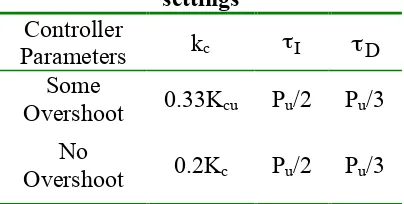
Modified Ziegler-Nichols Methods: For some control loops the measure of oscillation, provide by ¼ decay ratio and the corresponding large overshoots for set point changes are undesirable therefore more conservative methods are often preferable such as modified Z-N settings These modified settings that are shown in Table 2 are some overshoot and no overshoot.
Tyreus – Luyben Method:
The Tyreus-Luyben [10] procedure is quite similar to the Ziegler–Nichols method but the final controller settings are different. Also this method only proposes settings for PI and PID controllers. These settings that are based on ultimate gain and
Table 2- Modified Ziegler–Nichols settings
Controller
Parameters kc τI τD Some
Overshoot 0.33Kcu Pu/2 Pu/3
No
Table 3- Tyreus – Luyben settings
Controller kc τI τD
PI kcu/3.2 2.2Pu -
PID kcu/3.2 2.2Pu Pu/6.3
period are given in Table 3.
Like Z-N method this method is time consuming and forces the system to margin if instability. Many other algorithms have been proposed to solve these problems [7,8,9,17] by obtaining critical data (ultimate gain and frequency) under more acceptable conditions. One of these methods is damped oscillation method
Damped Oscillation Method:
This method is used for solving problem of marginal stability. The process is characterized by finding the gain at which the process has a damping ratio of ¼. and the frequency of oscillation at this point, Then similar the Ziegler-Nichols method these two parameters are used for finding the controller settings.
Define
Gd = Proportional gain at decay ratio of ¼
Pd= Period of oscillation
Having Gd and Pd and using Table 4, the
controller parameters are calculated.
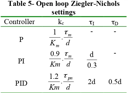
Open Loop Ziegler-Nichols Method: In this technique the process dynamics is modeled by a first order plus dead time model, given below:
1
Having the process model and using Table 5, the controller parameters can be obtained.
Table 4– Damped oscillation method relations
origin and double zeros at:
d
1
S
=
−
In using these formulas it is important to note that they are empirical and can be apply only to a limited range of dead time to time constant ratio. This means that they should not be extrapolated outside a range
of
m
d
τ of around 0.1 to 1.0.
The C-H-R Method:
This method that has proposed by Chien, Hrones and Reswich [1] is a modification of open loop Ziegler and Nichols method. They proposed to use “quickest response without overshoot” or “quickest response with 20% overshoot” as design criterion. They also made the important observation that tuning for set point responses and load disturbance responses are different.
To tune the controller according to the C- H-R method the parameters of first order plus dead time model are determined in the
same manner of the Z-N method. The controller parameters can then be determined from the Tables.6 and 7. The tuning rules based on the 20% overshoot design criterion are quite similar to the Z-N method. However when the 0% overshoot criteria is used, the gain and the derivative time are smaller and the integral time is larger. This means that the proportional action and the integral action, as well as the derivative action, are smaller.
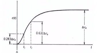
Cohen-Coon Method:
In this method the process reaction curve is obtained first, by an open loop test as shown in Figure 1, and then the process dynamics is approximated by a first order plus dead time model, with following parameters:
)
( 2 1
2 3
t t
m = −
τ (5)
m m
d =τ2 −τ (6) where
t1 = time at which ΔC=0.283 ΔCs
t1 = time at which ΔC=0.632 ΔCs
C = the plant output.
This method that proposed by Dr C. L. Smith [15] provides a good approximation to process reaction curve by first order plus dead time model
After determining of three parameters of km , τm and d, the controller parameters
can be obtained, using Cohen-Coon [14] relations given in Table 8. These relations were developed empirically to provide closed loop response with a ¼ decay ratio.
Figure 1- Estimating of parameters of first order plus dead time process model
Fertick Method:
This method uses a first order plus dead time model for the process:
1 + =
−
s ke s G
ds
m
τ
)
( (7)
then the Fertik controllability αF, must be calculated as:
ps d F
T T
d d
= + =
τ
α (8)
Td = d Tps =d+τ (9)
and then the normalized parameters should be read from the set of graphs shown in Figures (2) to (4). The parameters may be optimized for set point or disturbance changes. The PID controller is not recommended for those processes whose Fertik controlability is greater than 0.5. These processes are dominated by dead time. Notice that in Fertik method desired performance is minimizing ITAE with an 8% overshoot.
Ciancone and Marline Method:
Ciancone and Marlin (1992) [11] have developed a method that enable, engineer to obtain controller parameters by using some graphs to satisfy the control objective given below:
Minimizing IAE considering
1)
±
25
% change in the process model parameters.2) Limits on the variation of the manipulated variable.
These graphs are for both set point changes and load disturbances and for PI or PID controllers are available [11]. The method can provide controller parameters based on a process dynamic model. The model they used is a first order plus dead time model. In summery the tuning method consists of the following steps:
2) Calculate the ratio d /(τ+d), or fractio- nal dead time.
3) Select the appropriate graph depends on controller type (PI or PID) and type of input (set point or disturbance).
4) Determine the dimensionless tuning
values ⎟⎟
⎠ ⎞ ⎜⎜
⎝ ⎛
+
+ τ
τ τ τ
d d k
k I D
c , , from the graphs
5) Calculate the dimensional controller tuning. e.g. kc = (kc.k)/k
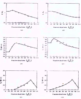
The graphs for PID controller are given in Figure (5).
Internal Model Control (IMC):
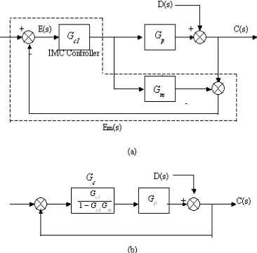
Morari and his coworkers [12] have developed an important new control system strategy that is called Internal Model Control or IMC. The IMC approach has two important advantages: (1) It explicitly takes into account model uncertainty and (2) It allows the designer to trade-off control system performance against control system robustness to process changes and modeling errors. The IMC approach is based on the block diagram shown in Figure 6. In this diagram Gp is the transfer function of the process
and Gm is the transfer function of the
process model. Also GcI is the IMC
controller transfer function. The equivalent
Figure 6- Internal Model Control (a) basic structure (b) equivalent feedback
feedback control system for IMC structure is also shown in Figure (6b).
The conventional controller transfer function can be related to the IMC controller as below:
m cI cI c
G G G G
− =
1
(10)
To make the control system more robust, the controller is cascaded with a filter of the following form:
n f f
s G
)
( 1
1 + =
τ (11)
Using IMC technique, Morari and Zafirion [12] proposed PID controller settings for a first order plus dead time model. These settings are given in Table (9).
The choice of the best ratio of λ/d must be based on performance and robustness considerations. Since for PI controller a zeroth order Pade approximation is used so it neglects the dead time so this causes that these settings does not provide responses with good performance. This can be remedies by incorporating the dead time in the internal model through other means and leads to the improved PI settings, shown in third row of Table (9)
Tuning Method for Minimum Error Integral Criteria:
As mentioned before tuning for ¼ decay ratio often leads to oscillatory responses and also this criterion considers only two points of the closed loop response (the first two peaks). The alternative approach is to develop controller design relation based on a performance index that considers the entire closed loop response.
Some of such indexes are as below
1) Integral of the absolute value of the error (IAE)
IAE=
∫
∞|e(t) .|dt0 (12)
2) Integral of the square value of the error (ISE)
ISE=
∫
∞e (t).dt0 2
3) Integral of the time weighted absolute value of the error (ITAE)
ITAE=
∫
∞ the error (ITSE)ITSE=
∫
∞t.e (t).dt0 2
(15)
Lopez et al [15] developed tuning formulas for minimum error criteria based on a first order plus dead time transfer function. The tuning relations for disturbance inputs have given in Table 10. These formulas indicate the same trend as the quarter decay ratio formulas except that the integral time depends more on the effective process time constant and less on the process dead time.
Again keep in mind that these formulas are empirical and should not be extrapolated beyond a range of d/τm of between 0.1 and 1.0
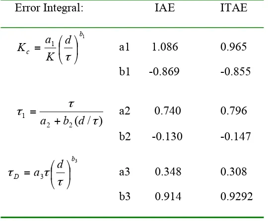
The tuning relations for set point tracking is given in Table 11 which has been developed by Rovira et al [15], who considered that the minimum ISE criterion was unacceptable because of its highly oscillatory nature. These formulas are also empirical and should not be extrapolated beyond the range of d/τm. between 0.1 to 1.0.
Simulation Study:
For simulation purpose the following systems have been considered:
Gp(s) =
As can be seen, the second order system is an under damped system. The simulation is carried out, using MATLAB (version 6.1)
software, and for two cases of set point tracking and load rejection. For all of these methods we have used a unit step like input for both set point and load changes. Notice that for IMC method, since we do not have an formula for second and third order systems with dead time so at first we estimate our system with a first order with dead time transfer function using the same method used for Cohen-Coon and minimum error tuning methods and then the settings in given Table (9).
Results and Conclusion:
The IAE values for different methods are given in Tables (12) and (13). Also to get a graphical insight, the values of IAE are plotted against tuning methods in Figures (7) through (12). Based on the simulation results given in these tables, the best performance (based on IAE values), and their corresponding tuning methods are summarized in Table 14.
Surprisingly it can be seen form Tables (12) and (13) that the minimum error tuning method for IAE (IAE method) does not result in minimum IAE for none of systems studied. But ISE method for first order and second order systems when we have disturbances gives the minimum IAE value. The possible reason for this can be the fact that the proposed controller settings for IAE methods have obtained empirically with a limited number of dyna-
Table 14-Summary of comparison of PID controller tuning methods based on
mic systems. Therefore it is probable that the typical systems studied here are different from those studied by Lopez et al [15].
For the case of set point tracking the closed loop Ziegler-Nichols method gives good and reasonable results, since the IAE value for this method is very close to the IAE value for the method that results in minimum IAE.. Also for load rejection, for third order system, closed loop Ziegler-Nichols method gives minimum IAE and for first and second order systems the IAE values for this method are not very far from minimum IAE values. This suggests that the traditional Ziegler-Nichols method can be used confidently for majority of systems, which confirms again wide applicability of this method.
References:
1) Astrom K,J, T. Hagllund; ”PID controllers Theory, Design and Tuning ”,2nd edition, Instrument Society of America,1994
2) Chen C.L., ”A Simple Method for Online Identification and Controller Tuning”, AIChe J ,35,2037 (1989)
3) Coughanowr D.R.; ”Process System Analysis and Control”,2nd edition McGraw-Hill,1991
4) Erickson K.T., J.L. Hedrick ; ”Plantwide Process Control” John Wiley & Sons,1999 5) Hang C.C., J.K. Astrom, W.K. Ho; ”Refine-
ments of Ziegler Nichols Tuning formula”, IEE Proceedings ,138(2),111(1991)
6) Jutan A.; ”A Comparison of Three Closed Loop Tuning Method Algorithms”, AIChe J,35,1912 (1989)
7) Krishnaswamy P.R., B.E Mary Chan.,and G.P, Rangaish; ”Closed- Loop Tuning of
Control Systems”, Chem. Eng.
Sci.42,2173(1987)
8) Lee J.; ”Online PID Controller Tuning For
A Single Closed Test”, AIChe
J,32(2),329(1989)
9) Lee J., W. Cho; ”An Improved Technique for PID Controller Tuning from Closed Loop Tests”, AIChe J,36,1891(1990)
10) Luyben W.L, M.L. Luyben; “Essentials of Process Control”, McGraw-Hill,1997
11) Marlin T.E.; ”Process Control”,2nd edition,,Mcgraw-Hill,2000
12) Morari M., E. Zafirion; ” Robust Process
Control”, Prentice-Hall, Englewood
Cliffs,NJ,1989
13) Ogata K.; ”Modern Control
Engineering”,3th edition, Prentice Hall 1997 14) Seborg, D.E., T.F. Edgar, D.A. Mellichamp; “Process Dynamics and Control”,
John Wiley & sons,1989 15) Smith,C.A., A.B. Copripio; ”Principles
and Practice of Automatic Process Control”, John Wiley & Sons,1985
16) Stephanopolous,G.; ”Chemical Process Control”, Prentice-Hall, 1984
17) Yuwata,M, D.E. Seborg; ”A new Method for Online Controller Tuning”, AIChe J,35,434(1982)
Table 6- Tuning relations for C-H-R method. Load rejection
Overshoot 0% 20%
Controller
Type Kc τI τD Kc τI τD
P
d K
3 .
0 m
m τ
__ __
d K
7 .
0 m
m τ
__ __
PI
d K
6 . 0 m
m τ
4d __
d K
m
m
τ 7 . 0
2.3d __
PID
d K
95 .
0 m
m τ
2.4d 0.42d
d K
2 .
1 m
m
τ
Table.7- Tuning relations for C-H-R method. Set point tracking
Table 8- Cohen-Coon controller settings
Controller
Table 9- IMC based real PID parameters for
ds
Table 10-Minimum error integral tuning formulas for disturbance inputs
Process Model: G(s)=
1 + s
e K ds
τ
Error Integral: ISE IAE ITAE
1
1
b
c
d
K a K
⎟ ⎟ ⎠ ⎞ ⎜ ⎜ ⎝ ⎛ =
τ
a1 1.495 1.435 1.357
b1 -0.945 -0.921 -0.947
2
2 1
b
d
a ⎟⎟ ⎠ ⎞ ⎜ ⎜ ⎝ ⎛
=
τ τ
τ a2 1.101 0.878 0.842
b2 0.771 0.749 0.738
3
3 b D
d
a ⎟
⎠ ⎞ ⎜ ⎝ ⎛ =
τ τ
τ a3 0.560 0.482 0.381
b3 1.006 1.137 0.995
Table 11-Minimum error integral tuning formulas for set point changes
Process Model:
1 )
(
+ =
s e K s G
ds
τ
Error Integral: IAE ITAE
1 1
b
c
d
K a
K ⎟
⎠ ⎞ ⎜ ⎝ ⎛ =
τ a1 1.086 0.965 b1 -0.869 -0.855
) / ( 2 2 1
τ τ τ
d b a +
= a2 0.740 0.796
b2 -0.130 -0.147
3
3
b
D
d a ⎟
⎠ ⎞ ⎜ ⎝ ⎛ =
τ τ
τ a3 0.348 0.308
Table 12 – IAE values for various tuning methods, Set Point Tracking
No .
System Method
First Order System 1
Second Order System 2
Third Order System 3
Simulation Time
10 20 30
1 Z-N (Closed Loop) 0.47 2.25 4.26
2 Modified Z-N
(some overshoot) 0.71 1.95 7.53
3 Modified Z-N
(no overshoot) 0.71 2.3 9.46 4 Tyreus-Luyben 1.4 4.87 7.6 5 Damped Oscillation 0.44 2.13 5.7
6 Fertik 0.47 3.56 12.22
7 Ciancone 0.59 2.2 9.29
8 Z-N (Open l.oop) 0.51 5.06 8.77
9 C-H-R
(0%overshoot) 0.5 2.51 4.28 10 C-H-R
(20%overshoot) 0.69 3.39 11.9 11 Cohen Coon 0.67 2.29 4.36
12 IAE 0.72 2.26 6.35
13 ITAE 0.68 2.12 5.58
14 IMC 0.6 2.16 4.41
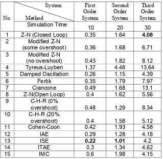
Table 13 – IAE values for various tuning methods, Load Rejection
No.
System Method
First Order System
Second Order System
Third Order System
Simulation Time
10 20 30 1 Z-N (Closed Loop) 0.35 1.64 4.08
2 Modified Z-N
(some overshoot) 0.36 1.68 6.71 3 Modified Z-N
(no overshoot) 0.43 1.82 8.12 4 Tyreus-Luyben 1.37 4.48 13.64 5 Damped Oscillation 0.26 1.15 4.39
6 Fertik 0.35 1.79 7.97
7 Ciancone 0.49 1.68 13.1
8 Z-N(Open Loop) 0.4 1.62 5.56 9 C-H-R (0%
overshoot) 0.48 1.29 8.34 10 C-H-R (20%
overshoot) 0.4 1.58 5.12 11 Cohen-Coon 0.42 1.93 4.58
12 IAE 0.29 1.28 4.18
13 ISE 0.22 1.01 4.2
Figure 2- Fertik controller gain for Figure 3- Fertik controller integral for PID controller time for PID controller
Figure 4- Fertik derivative time for PID controller
Figure 5- Ciancone correlations for determining tuning constants, PID algorithm. For disturbance response (a) controller gain. (b) Integral time. (c) derivative time. For set point response: (d) controller gain (e) integral time (f)
0 0.5 1 1.5
1 3 5 7 9 11 13
Mehtod Number*
IA
E
Figure 7- IAE values against tuning method for first order system
(set point tracking)
* Refer to Table 12
Figure 9- IAE values against tuning method for third order system
(set point tracking)
* Refer to Table 12
0 1 2 3 4 5
1 3 5 7 9 11 13 15
Mehtod Number*
IA
E
Figure 11- IAE values against tuning method for second order system
(load rejection)
*Refer to Table 13
0 1 2 3 4 5 6
1 3 5 7 9 11 13
Mehtod Number*
IA
E
Figure 8- IAE values against tuning method for second order system
(set point tracking)
*Refer to Table 12
0 0.5 1 1.5
1 3 5 7 9 11 13 15
M e htod Num be r *
IA
E
Figure 10- IAE values against tuning method for first order system
(load rejection)
*Refer to Table 13
0 5 10 15
1 3 5 7 9 11 13 15
Mehtod Number
IA
E
Figure 12- IAE values against tuning method for third order system
(load rejection)