JMEA Volume 8 Number 2 February 2018 Ser

(1)

(2)

Volume 8, Number 2, February 2018 (Serial Number 71)

Journal of Mechanics

and

Automation

Engineering

Dav i d

David Publishing Company www.davidpublisher.com

(3)

Publication Information:

Journal of Mechanics Engineering and Automation is published monthly in hard copy (ISSN 2159-5275) and online (ISSN 2159-5283) by David Publishing Company located at 616 Corporate Way, Suite 2-4876, Valley Cottage, NY 10989, USA.

Aims and Scope:

Journal of Mechanics Engineering and Automation, a monthly professional academic journal, particularly emphasizes practical application of up-to-date technology in realm of Mechanics, Automation and other relevant fields. And articles interpreting successful policies, programs or cases are also welcome.

Editorial Board Members:

Andrea Mura (Italy), Bin Li (Canada), Dumitru Nedelcu (Romania), Guian Qian (Switzerland), Ionel Staretu (Romania), Isak Karabegovic (Bosnia and Herzegovina), Ivanov Konstantin Samsonovich (Kazakhstan), Jianhua Zhang (China), Dr. Kishore Debnath (India), Mohammad Mehdi Rashidi (Iran), Dr. Mohamed Ali (Saudi Arabia), Olga Roditcheva (Sweden), Pak Kin Wong (Macao), Peng-Sheng Wei (Taiwan), Rodrigo L. Stoeterau (Brazil), SADETTIN ORHAN (Turkey), Sergio Baragetti (Italy), Wei Min Huang (Singapore), Zongwei Xu (China)

Manuscripts and correspondence are invited for publication. You can submit your papers via web submission, or E-mail to mechanics@davidpublishing.com. Submission guidelines and web submission system are available at http://www.davidpublisher.com.

Editorial Office:

616 Corporate Way, Suite 2-4876, Valley Cottage, NY 10989, USA Tel: 1-323-984-7526, 323-410-1082; Fax: 1-323-984-7374, 323-908-0457 E-mail: mechanics@davidpublishing.com

Copyright©2018 by David Publishing Company and individual contributors. All rights reserved. David Publishing Company holds the exclusive copyright of all the contents of this journal. In accordance with the international convention, no part of this journal may be reproduced or transmitted by any media or publishing organs (including various websites) without the written permission of the copyright holder. Otherwise, any conduct would be considered as the violation of the copyright. The contents of this journal are available for any citation. However, all the citations should be clearly indicated with the title of this journal, serial number and the name of the author.

Abstracted / Indexed in: Google Scholar

Chinese Database of CEPS, Airiti Inc. & OCLC

Chinese Scientific Journals Database, VIP Corporation, Chongqing, China CSA Technology Research Database

CrossRef

Norwegian Social Science Data Services (NSD), Norway CNKI, China

Ulrich’s Periodicals Directory

Subscription Information:

Price (per year): Print $520; Online $320; Print and Online $600

David Publishing Company

616 Corporate Way, Suite 2-4876, Valley Cottage, NY 10989, USA Tel: 1-323-984-7526, 323-410-1082; Fax: 1-323-984-7374, 323-908-0457 E-mail: order@davidpublishing.com

Digital Cooperative Company: www.bookan.com.cn

David Publishing Company www.davidpublisher.com

(4)

Jour na l of M e cha nic s

Engine e ring a nd

Aut om at ion

Volume 8, Number 2, February 2018 (Serial Number 71)

Techniques and Methods

43 Review of Metal AM Simulation Validation Techniques

Aaron Flood and Frank Liou

53 A Brief Tour on Exotic Control Objectives in Robotics

Rafael Kelly and Carmen Monroy

60 Optimizing Hot Forging Process Parameters of Hollow Parts Using Tubular and Cylindrical Workpiece: Numerical Analysis and Experimental Validation

Angela Selau Marques, Luana De Lucca de Costa, Rafael Luciano Dalcin, Alberto Moreira Guerreiro Brito, Lirio Schaeffer and Alexandre da Silva Rocha

Investigation and Analysis

71 Definition of Stationarity Based on Monitoring the Uncertainty at Real Measurement Conditions

Alois Heiss and Woelfel Engineering Group

82 Strengthening Effects of Niobium on High Strength Rebars

Zhang Yongqing, Guo Aimin and Yong Qilong

92 Estimating Emotion for Each Personality by Analyzing BVP

(5)

(6)

Journal of Mechanics Engineering and Automation 8 (2018) 43-52 doi: 10.17265/2159-5275/2018.02.001

Review of Metal AM Simulation Validation Techniques

Aaron Flood and Frank Liou

Department of Mechanical and Aerospace Engineering, Missouri University of Science and Technology, Rolla 65409, USA

Abstract: Due to the complexity of metal AM (additive manufacturing), it can require many trial runs to obtain processing parameters which produce a quality build. Because of this trial and error process, the drive for simulations of AM has grown significantly. A simulation only becomes useful to researchers if it can be shown that it is a true representation of the physical process being simulated. Each process being simulated has a different method of validation to show it is an accurate representation of the process. This paper explores the various methodologies for validation of laser-based metal AM simulations, focusing mainly on the modeling of the thermal processes and other characteristics derived from the thermal history. It will identify and explain the various validation techniques used, specifically looking at the frequency of reported use of each technique.

Key words: AM simulation, simulation validation, heat transfer modeling, stress modeling, micro-structure modeling.

1. Introduction



AM (additive manufacturing) is a complex process and many have attempted to generalize the process using mathematical models. In order to show the validity of each model, researchers have developed methods to compare the results from these simulations to experiments which can be performed. Each aspect of the AM process which is being simulated will have a different technique for validation. The main phenomena of AM which have been studied are heat transfer, induced stress, and microstructure. For each of these phenomena, the various validation techniques which have been used in literature will be investigated including a brief description of the technique fundamentals.

There are two main methods of validation for the modeling of the thermal history, instrumental and indirect. The instrumental methods utilize a hardware setup to directly measure the temperature of the process at a specific location. Whereas the indirect methods compare a different physical characteristic, such as melt pool depth, which is linked to the temperature, this is then used to validate the temperature profile.

Corresponding author: Aaron Flood, PhD candidate, research field: metal additive manufacturing simulation.

To validate the stresses which are induced on the part, qualitative and quantitative approaches have been utilized. To qualitatively validate the results, some have looked for the generation of cracks and compared these results to a simulation. This validation can give a gross comparison of the simulation and experiments. A simple method of gathering a quantitative comparison is to measure the distortion of the final part. This can either be done using a laser displacement sensor, in situ, or a 3-D scanner after the deposition is complete. These results, though more precise than crack generation, are not extremely precise. To precisely measure the strain, it is necessary to gather a diffraction pattern, either with X-rays or neutrons, for the part. This allows for the precise locations of the atoms to be known which gives the exact values for the strain in the part.

Due to the drive for AM from the aerospace industry, many researchers are focusing on Ti-64 (Ti-6Al-4V) as their material of choice. Therefore that will be the focus of the microstructure section of this paper. Even though the focus is Ti-64, all the methods which are presented can be generalized to any metal. The first method of comparison is to compare the phase which occurs, usually on a pixel by pixel basis or a voxel by voxel basis for 3-D. This will give a general comparison and limited quantitative comparison of the experiment and simulation. If a more detailed comparison is desired,

D

(7)

then in addition to the phase the grain sizes can be compared. This comparison is usually made by comparing the size distribution of the phases.

2. Heat Transfer Validation Techniques

The most fundamental, and first developed, process in AM which has been modeled is the flow of heat through the part. This problem was first tackled by researchers focusing on simulating the welding process, and much can be derived from their work. A very extensive review was done by Mackwood and Crafer [1] from which key elements can be utilized. The first numerical solutions which can be applied to the problem of AM, by Mazumder and Steen [2], created a 3-D finite difference model to simulate a Gaussian laser on a semi-infinite workpiece. Their model did not include temperature dependent material properties, which was later remedied by Chande and Mazumder [3]. This later iteration also accounted for latent heat of phase change which has recently proven to be an important aspect of AM simulations. The last simulations developed, which are the most applicable to AM, are for multi-pass welding by Reed and Bhadeshia [4], Lindgreen et al. [5], and Frewin and Scott [6]. In these models, the laser is passed over the same area multiple time to determine the heat flow due to the multiple passes. These simulations were the first time that “quiet” elements were utilized. These elements are considered inactive until the part has been built up to their location. At that time, they are activated and are included in the simulation. This model has been the foundation that most AM simulations have been built upon.

In order to validate these models, thus far in the literature, there have been two approaches. The first is to validate the thermal model with an instrument equipped to measure temperature. If this has not been done, then the researchers will measure another physical characteristic of the build and use that to show the model’s validity. A representative set of papers have been presented in Table 1.

Table 1 Breakdown of validation techniques. Instrument validated Physical char. validated IR/CCD camera [7-10] Melt pool depth [11-13] Pyrometer [14, 15]

Thermal couple [15-17]

These papers show that more attempts have been made to validate the models using instrumental validation as opposed to using another physical characteristic. This is most likely due to the direct link between the measured value and the simulated value. When using another physical characteristic, it is necessary to know the exact linkage between the trait being measured and the one being simulated. For this reason, there are more opportunities for error and false validation, or rejection, of a given model. From the literature reviewed, there are three prominent instruments which have been used to validate the models.

(8)

Review of Metal AM Simulation Validation Techniques

45

using a pulsed laser, the skin temperature can spike very rapidly which can result in inaccurate measurements.

, (1)

1 ⁄∑ 1 (2)

The next instrument most commonly used is a pyrometer, which is a non-contact spot measurement which can be used in-situ. This results in the ability to measure the average temperature of a specific area. This is not as useful as cameras previously presented due to the lack of resolution. However, because of their simplicity, it is possible to create a mathematical model to predict the pyrometer output. This can be done by knowing the power of the thermal radiation which returns to the pyrometers and is shown in Eq. (1) [20], where I(λ, T), is the spectral distribution of the blackbody emissive power given Planck’s radiation law. It is possible to then integrate Eq. (1), assuming that the laser is a Gaussian heat source and that the pyrometer is sampling a 1 mm radius, it is possible to solve for the effective temperature that the pyrometer reads, Eq. (2), where h is Planck’s constant, c is the speed of light, λ is the wavelength of the emitted radiation, σ is Stefan-Boltzmann constant, n is the number of small sampling areas within the pyrometer viewing area, and

Ti is surface temperature within the small n areas.

This has allowed for Dia et al. [14] to create a simulation which includes a pyrometer to control the laser power. This simulation can predict the changes that the pyrometer will make to the laser power, for a closed loop system, to keep a constant melt pool size. The last method found in the literature to measure the temperature directly utilizes thermocouples, which are contact spot measurements. The fact that they must be fixed, welded in most cases, to the surface makes them impractical for some applications, such as powder bed process. In addition, they will only record the average temperature of a specific location. Therefore, to obtain an accurate representation of the temperature

profile, several thermocouples need to be placed on the working surface. Another downfall with thermocouples is their inability to measure the melt pool temperature. Since they need to be fixed to the surface, if an attempt is made to measure the melt pool they will become detached from the substrate and the data will be invalid. For these reasons, current researchers have only used thermocouples as a secondary validation technique and utilize another technique for the main source of data.

Besides these direct methods of validating the thermal modeling, some researchers have taken the approach of measuring a more easily attained data set and compared that to the simulation, namely the melt pool size and the shape of the build. In this method a simple surface laser heating simulation and experiment are performed, where the laser is simply used to melt a track on the surface of the substrate. In the experiments, a slice is taken perpendicular to the laser path which is then analyzed, typically with an optical microscope. This allows for the width and depth of the melted region to be measured, as seen on the left image in Fig. 1. In the simulation, since the temperature is tracked for each element, it is possible to flag elements which have melted, this is done in the right image in Fig. 1 by changing their color to red. In addition to the use of the surface laser heating, some have simulated a single track build, which can be seen in Fig. 2.

Fig. 1 Validation of thermal analysis by comparing melt pool dimensions of experiment (left) and simulation (right) [12].

(9)

Table 2 Applicability of validation techniques to basic AM processes.

Table 3 Highest accuracy reported of validation techniques to basic AM processes.

Response Time Resolution

IR/CCD camera 800 fps [7] 10.9 um2 [8]

Pyrometer 3 mm2_[14]

Thermal couple 0.2 mm2_[15]

*Values not reported are left blank.

This indirect method of validation can typically be done without specialty equipment. However, this method of validation introduces new complications which can hide, or skew, the results. Since the material is melted, the flow of the molten material dictates the shape of the melt pool. For that reason, this validation technique requires that both the thermal and fluid models are correct. Therefore, the direct methods are simpler to implement than the indirect methods.

In general, these methods all have different

applicability to the various metal AM processes. As can be seen in Table 2, all the methods of validation are applicable to DED (directed energy deposition) metal AM. When working with a powder bed process, on the contrary, it is impossible to use a thermocouple as previously stated. For this method of metal AM, it is necessary to use one of the non-contact methods. When looking at the accuracy of the methods, displayed in Table 3, the camera system will usually have the highest resolution and response time, but will also be the most expensive. Therefore, it is necessary to balance the cost and the accuracy needed.

3. Stress Validation Techniques

Inherent in AM processes, is a cyclic heating which leads to stresses being induced. The stressing process has been divided into four stages by Ding et al. [21].

Stage A occurs when the heat source approaches the

location of interest on the part. This stress is compressive since the volume under the heat source is expanding. This compressive stress is elastically compensated for by the material until the compressive yield stress limit is surpassed. When the compressive yield limit is surpassed, stage B takes place. In this stage, plastic flow of material occurs and the compressive stress is reduced. Stage C has begun when the material begins to cool which results in tensile stress. These stresses are caused by the contraction of the surrounding material. They remain elastic until the tensile yield stress is surpassed. The final stage of stress is stage D, which occurs when the tensile yield limit is surpassed and plastic flow begins. These stresses can all be derived from the thermal history of a specific location and its neighbors. Due to the difficulty of measuring the stress, only a few methods have been used throughout literature as displayed in Table 4.

One of the simplest, though not accurate method, is to observe the creation of cracks within the part and compare that to simulation results. This method, used by Zhu et al. [9], is simple and can be done without any specialty equipment. This method, however, due to its lack of precision, can only be used to qualitatively verify that a simulation is giving results which generally agree with the experiment. This method cannot be used to quantitatively validate a mathematical model.

If a more refined approach is needed Liu et al. [22] have looked at build plate deformation as a link between the simulation and the experiment. Thus far in the literature, this has been implemented by using a laser displacement sensor or a 3-D scanner to measure the distortion which occurs in the final part. To use a laser displacement sensor, as shown in Fig. 3, one edge

(10)

47

Fig. 3 Experimental setup using laser displacement sensor to measure distortion [23].

of the build plate is clamped creating a cantilever, and the sensor is used to monitor the free end. This edge of the build plate is monitored in real time to determine the fluctuations that occur during the build. These fluctuations are then correlated to the distortions which are seen in the simulation. When done correctly, the stress which occurs in the part can be correlated to the simulation to show the accuracy of the simulation. This method, in addition to measuring the stresses as they occur, has the added capability to measure the residual stresses which build up throughout the entire process. One problem with this setup is that the depositions location on the substrate is critical for accurate results. This is simple in the simulation, however, in the experimental setup, this can prove challenging. The other method of measuring the induced stresses is to build the part and upon removal from the machine, to use a 3-D scanner to measure distortions. This will give the final dimensions of the part and a more complete picture can be gained using this approach.

Each of these approaches has its advantages. If a full picture of the part is needed, then a 3-D scanner should be utilized. This is because the scanner inspects the whole part, or at least a larger section of the part, compared to the laser displacement sensor which only monitors a single point.

However, if more accurate results are needed, then a laser displacement sensor should be used. The laser sensor used by Heigel et al. [17] reports an accuracy of ±1 µm, whereas the 3-D scanner used by Denlinger et al. [24] reported an accuracy of ±500 µm.

Another method of obtaining the distortion, or the surface stresses induced, of the part is DIC. The process of DIC uses a camera to observe the part and sense any motion which is induced on the part. Pan et al. [29] describe how this method tracks points which are placed on the part to determine their relative motion to calculate the stresses and distortion a part endures. An example of how the points move can be seen in Fig. 4. This method will inherently give the distortion of the part. However, Wu et al. [25] showed that it is possible to precisely determine the surface level stresses which are induced on the part. This is done by selectively stress relieving the part through sectioning, hole drilling, or slitting. These methods allow for the distortion that occurs to be related back to the stress which the part is experiencing. The main drawback to this method of validation is that it is a destructive method. However, one of the main advantages of this method is that the resolution is limited by the camera which is being used. The motion of the material is measured in pixels on the camera. That results in the ability to have a fine resolution if a high-resolution camera is used. The resolution of the camera can also be supplemented by attaching the camera to a microscope. This technique can greatly increase the detail which can be observed with the DIC method.

(11)

Fig. 4 Schematic showing displacement of tracking points in DIC [29].

will move the atoms. The difference in the diffraction patterns directly correlates to the distance that the atoms shifted. This motion of atoms is known as the strain which can then be converted to stress using Hooke’s law.

This method of determining the stress locally allows for a direct correlation between the experiment and simulation. The choice of neutron or X-ray is based mainly on availability to the researchers. The use of XRD (X-ray diffraction) is much more widely available to researchers and therefore generally a more cost-effective method, whereas the use of neutrons is only done in specific facilities. One of the downfalls of these strain measurements is their inability to be used in-situ. Therefore the measurements are only of the final stresses. In addition to the localized strain, Ding et al. [16] have used the aforementioned 3-D scanners to further verify the simulations results.

4. Microstructure Validation Techniques

Due to its many desirable characteristics, namely its high strength to weight ratio and corrosion resistance, Ti-64 has been the focus of many researchers and leaders in industry. Because of this previous body of knowledge, this section will focus on Ti-64. However, these techniques can be applied to most metals. In many metals, and in particular Ti-64, the microstructure is critical to obtain optimal strength. Because of this, many researchers have developed

models to determine the microstructure of an AM build.

To understand the modeling of the microstructure of Ti-64, it is necessary to study the microstructures that can occur. Ti-64, according to Kelly [31], has a microstructure which is a combination of a BCC (body-centered cubic), which is denoted as a β phase, and an HCP (hexagonally closed packet), which is denoted as an α phase. These phases will coexist within the Ti-64 part and the quantities and sizes will depend on the maximum temperature and cooling rate at a specific location. At room temperature, the typical micro-structure is α + β. If the material’s temperature is raised higher than the beta transus temperature the material will transition into pure beta phase. As the material cools, the alpha phase will reappear and the cooling rate will dictate which alpha phases occur. This is shown graphically in Fig. 5. If the cooling rate is fast then the resulting alpha phase will be Martensitic (α0)

or Massive (αm). These phases will appear

intra-granularly and on the grain boundaries respectively. On the contrary, if the cooling rate is slow then the resulting micro-structure will start with Allotriomorphic (αGB) on the grain boundaries

followed by primary-alpha (αP), which is simply any

(12)

49

beta transus temperature, some of the αP will convert to

β. When this material then cools, the new phase created is called secondary-alpha (αS). This secondary phase

becomes critical in AM due to the constant reheating

from the layer by layer manufacturing strategy. Based on this understanding of the micro-structure evolution there are a few methods of quantifying, and therefore validating, a simulation which are outlined in Table 5.

Fig. 5 Phase transformations which occur in Ti-64 [31].

(13)

Table 5 Frequency of micro-structure analysis techniques. Element Wise Comparison [32]

Phase Volume Comparison [33, 34] Grain Size Distribution [9, 33, 35]

In the first simulation method, by Kelly et al. [32], the elements are only allowed to be one of the various phases. Based on the elements thermal history, it is denoted as either beta or one of the alpha phases. This allows for a very general comparison with experimental results. When a thin wall is built, it can be sliced perpendicular to the laser scanning direction. This slice can then be observed with the SEM (scanning electron microscope). These images will then produce distinct regions, as shown in Fig. 7, of each phase which can be compared to simulations.

This simplified method is a fundamental start but is very lacking. Metallurgy has shown that the grain size, morphology, and distribution of fine particles are just as important to the mechanical properties as the phase itself. Therefore, Murgau et al. [34] have attempted to model the grain size along with the phase. The simplest of these validations use the volume percent of each of the phases. To ensure that their solution is robust, several cooling rates were modeled and compared to experimental results. When several cooling rates simulated matched experimental results, the simulation was considered correct, which is illustrated in Fig. 8.

Another method of validating the micro-structure is by comparing the size distribution of the alpha phase, which was done by Charles [35]. To compare the size distribution of the alpha phase, the average width of the alpha phases can be calculated and this can be used to compare the simulation to the experimental data. In order to be more rigorous Katzarov et al. [33] created a histogram of the sizes of the alpha phase in addition to the use of the volume percent of the phases. All in all, if a more detailed and rigorous validation technique is used the simulation can be more trusted.

Fig. 7 Phase layers of Ti-64 produced via thin wall deposition [32].

(14)

51

5. Conclusions

This paper presents the main validation techniques in literature for the validation of thermal modeling of metal AM and other attributes which are related to the thermal history. The heat transfer in the build can be measured using either direct or indirect means. The direct means include the use of cameras, pyrometers, and thermocouples. These methods give a direct link between the mathematical models and the experimental data. The indirect methods of validation use the melted track dimensions to show that the simulation is correct. This method relies heavily on the fluid model being correct as well as the correctness of the thermal model. Because of this, it can be preferred to use a direct method of measuring the heat flow.

Closely linked to the thermal history are the stresses induced in the build. To verify the modeling of stresses developed during a build, some have used the presence of cracks. This is only a rough correlation and to be more precise the parts distortion, during and after the build, can be analyzed, along with distortions which occur after selective sectioning to reveal the induced stresses, lastly to directly measure the strain diffraction that needs to be utilized to measure the shift of the atoms within the material.

In addition to the stress, the microstructure of Ti-64 is mainly dependent on the thermal history. The validation of this simulation can take a crude form of validation based solely on the phase present. A more rigorous approach involves calculating the percent volume of each of the phases and comparing these values. In addition, the size distribution of a phase can be found which can be used for more robust validation. All in all, the validation of simulation is very critical and sometimes an overlooked step. The selection of a validation technique must be appropriate for the simulation which is being created.

References

[1] Mackwood, A., and Crafer, R. 2005. “Thermal Modelling of Laser Welding and Related Processes: A Literature

Review.” Optics & Laser Technology 37: 99-115. [2] Mazumder, J., and Steen, W. 1980. “Heat Transfer Model

for CW Laser Material Processing.” Journal of Applied Physics 51: 941-7.

[3] Chande, T., and Mazumder, J. 1981. “Heat Flow during CW Laser Materials Processing.” In Lasers In Metallurgy: Proceedings of a Symposium, TMS-AIME, 165-77. [4] Reed, R., and Bhadeshia, H. 1994. “A Simple-Model for

Multi-pass Steel Welds.” Acta Metall Mater 42: 3663-78. [5] Lindgren, L., Runnemalm, H., and Nasstrom, M. 1999.

“Simulation of Multi-pass Welding of a Thick Plate.” International Journal For Numerical Methods In Engineering 44: 1301-16.

[6] Scott, D. A., and Frewin, M. R. 1999. “Finite Element Model of Pulsed Laser Welding.” Weld. J. 78 (1): 15-22. [7] Hu, D., and Kovacevic, R. 2003. “Sensing, Modeling and

Control for Laser-Based Additive Manufacturing.” International Journal of Machine Tools and Manufacture 43: 51-60.

[8] Kolossov, S., Boillat, E., Glardon, R., Fischer, P., and Locher, M. 2004. “3D FE Simulation for Temperature Evolution in the Selective Laser Sintering Process.” International Journal of Machine Tools and Manufacture 44: 117-23.

[9] Zhu, G., Zhang, A., Li, D., Tang, Y., Tong, Z., and Lu, Q. 2011. “Numerical Simulation of Thermal Behavior during Laser Direct Metal Deposition.” The International Journal of Advanced Manufacturing Technology 55 (9-12): 945-54.

[10] Zeng, K., Pal, D., and Stucker, B. E. 2012. “A Review of Thermal Analysis Methods in Laser Sintering and Selective Laser Melting.” In Proceedings of the Solid Freeform Fabrication Symposium, 796-814.

[11] Contuzzi, N., Campanelli, S. L., and Ludovico, A. D. 2011. “3D Finite Element Analysis in the Selective Laser Melting Process.” International Journal of Simulation Modelling 10 (3): 113-21.

[12] Khairallah, S. A., and Anderson, A. 2014. “Mesoscopic Simulation Model of Selective Laser Melting of Stainless Steel Powder.” Journal of Materials Processing Technology 214 (11): 2627-36.

[13] Tang, Q., Pang, S., Chen, B., Suo, H., and Zhou, J. 2014. “A Three Dimensional Transient Model for Heat Transfer and Fluid Flow of Weld Pool during Electron Beam Freeform Fabrication of Ti-6-Al-4-V Alloy.” International Journal of Heat and Mass Transfer 78: 203-15.

(15)

[15] Peyre, P., Aubry, P., Fabbro, R., Neveu, R., and Longuet, A. 2008. “Analytical and Numerical Modelling of the Direct Metal Deposition Laser Process.” Journal of Physics D: Applied Physics 41 (2): 025403.

[16] Ding, J., Colegrove, P., Mehnen, J., Ganguly, S., Almeida, P. M. S., Wang, F., and Williams, S. 2011. “Thermo-mechanical Analysis of Wire and Arc Additive Layer Manufacturing Process on Large Multi-layer Parts.” Computational Materials Science 50 (12): 3315-22. [17] Heigel, J. C., Michaleris, P., and Reutzel, E. W. 2015.

“Thermo-mechanical Model Development and Validation of Directed Energy Deposition Additive Manufacturing of Ti-6Al-4V.” Additive Manufacturing 5: 9-19.

[18] Wegner, A., and Witt, G. 2011. “Process Monitoring in Laser Sintering Using Thermal Imaging.” In Proceedings of the Solid Freeform Fabrication Symposium, 405-14. [19] Fischer, P., Locher, M., Romano, V., Weber, H. P.,

Kolossov, S., and Glardon, R. 2004. “Temperature Measurements during Selective Laser Sintering of Titanium Powder.” International Journal of Machine Tools and Manufacture 44 (12-13): 1293-6.

[20] Zhang, Y. 1998. “Thermal Modeling of Advanced Manufacturing Technologies: Grinding, Laser Drilling, and Solid Freeform Fabrication.” PhD thesis, University of Connecticut.

[21] Ding, J., Colegrove, P., Mehnen, J., Williams, S., Wang, F., and Almeida, P. S. 2014. “A Computationally Efficient Finite Element Model of Wire and Arc Additive Manufacture.” International Journal of Advanced Manufacturing Technology 70 (1-4): 227-36.

[22] Liu, H., Sparks, T. E., and Liou, F. W. 2013. “Numerical Analysis of Thermal Stress and Deformation in Multi Layer Laser Metal Deposition Process.” In Proceedings of the Solid Freeform Fabrication Symposium, 577-91. [23] Gusarov, A. V., Pavlov, M., and Smurov, I. 2011.

“Residual Stresses at Laser Surface Remelting and Additive Manufacturing.” Physics Procedia 12: 248-54. [24] Denlinger, E. R., Irwin, J., and Michaleris, P. 2014.

“Thermo-mechanical Modeling of Additive Manufacturing Large Parts.” Journal of Manufacturing Science and Engineering 136 (6): 061007.

[25] Wu, A. S., Brown, D. W., Kumar, M., Gallegos, G. F., and King, W. E. 2014. “An Experimental Investigation into Additive Manufacturing-Induced Residual Stresses in 316

L Stainless Steel.” Metallurgical and Materials Transactions A: Physical Metallurgy and Materials Science 45 (13): 6260-70.

[26] King, W., Anderson, A. T., Ferencz, R. M., Hodge, N. E., Kamath, C., and Khairallah, S. A. 2015. “Overview of Modelling and Simulation of Metal Powder Bed Fusion Process at Lawrence Livermore National Laboratory.” Materials Science and Technology 31 (8): 957-68. [27] Yadroitsava, I., and Yadroitsev, I. 2013. “Residual Stress

in Metal Specimens Produced by Direct Metal Laser Sintering.” In Proceedings of the Solid Freeform Fabrication Symposium, 1689-99.

[28] Shah, K., Izhar, U. H., Shah, S. A., Khan, F. U., Khan, M. T., and Khan, S. 2014. “Experimental Study of Direct Laser Deposition of Ti-6Al-4V and Inconel 718 by Using Pulsed Parameters.” The Scientific World Journal 2014: 841549.

[29] Pan, B., Qian, K., Xie, H., and Asundi, A. 2009. “Two-Dimensional Digital Image Correlation for in-Plane Displacement and Strain Measurement: A Review.” Measurement Science and Technology 20 (6).

[30] Fitzpatrick, M. E., Fry, A. T., Holdway, P., Kandil, F. A., Shackleton, J., and Suominen, L. 2005. “Determination of Residual Stresses by X-ray Diffraction—Issue 2.” Measurement Good Practice Guide (52): 74.

[31] Kelly, S. M. 2004. “Thermal and Microstructure Modeling of Metal Deposition Processes with Application to Ti-6Al-4V.” PhD thesis, Virginia Polytechnic Institute and State University.

[32] Kelly, S. M., Babu, S. S., David, S. A., Zacharia, T., and Kampe, S. L. 2004. “A Thermal and Microstructure Model for Laser Deposition of Ti-6Al-4V.” 45-52.

[33] Katzarov, I., Malinov, S., and Sha, W. 2002. “Finite Element Modeling of the Morphology of β to α Phase Transformation in Ti-6Al-4V Alloy.” Metallurgical and Materials Transactions A 33A: 1027-40.

[34] Murgau, C. C., Pederson, R., and Lindgren, L. E. 2012. “A Model for Ti–6Al–4V Microstructure Evolution for Arbitrary Temperature Changes.” Modeling and Simulation in Materials Science and Engineering 20: 055006.

(16)

Journal of Mechanics Engineering and Automation 8 (2018) 53-59 doi: 10.17265/2159-5275/2018.02.002

A Brief Tour on Exotic Control Objectives in Robotics

Rafael Kelly1 and Carmen Monroy

1. DET-DFA, Division de Fisica Aplicada, CICESE, Carretera Ensenada-Tijuana No. 3918, Zona Playitas, Ensenada, B.C., 22860,

Mexico

2

2. ISEP–Sistema Educativo Estatal, Zona 01, Ensenada, B.C., 22800, Mexico

Abstract: Formulation of control objectives is a key issue in automatic control systems design. Although at first sight the desired goal (control objective) of a control system seems to be a trivial and obvious matter, for effectiveness of some high level robotic tasks, unusual exotic control objectives may be required. This paper presents a review of some exotic control objectives useful in robotics, such as velocity field control objective and range control objective. The paper also proposes a novel confinement control objective. The usefulness of these exotic control objectives may appear in safe robot-human interaction and self-protection of robots against collisions.

Keywords: Control objective, robot, robot-human, confinement, range, velocity field, TEFDA (total energy function with damping assignment), exotic.

1. Introduction to Elements of Automatic

Control of Robots



It is recognized that many standard robot manipulator applications such as parts positioning/handling, painting, and pick-and-place can be well accomplished by standard well-established control systems such as PID control or compute-torque control [1-3]. Notwithstanding, some other new and more challenging robotic tasks such as safe robot-human interaction, multi-robot cooperation/competition, robot self-protection against auto-collisions, tasks under multi-sensor fusion, and robot tasks under embedded dynamic and unstructured environments are unable to be done by using such standard textbook control systems, hence this paper claims that a broad spectrum for innovation in novel Robots as a kind of amazing autonomous machines are equipped with digital computer implemented automatic control system (the “robots brain”). So, the effectiveness, applicability and accuracy of robots depend strongly on features of the underlying control system.

Corresponding author: Rafael Kelly, Ph.D., professor, research fields: automatic control, robotics,

powerful high task-level control system is still open in robotics sheltered under the so-called in this paper as exotic control objectives. This paper is an enhanced version of an early one presented in Ref. [4].

This paper adopts the following definition of robot. Definition 1—Robot

♦

Remark 1: This definition 1 includes both mobile robots as well as robot manipulators.

Remark 2: Although some engineers use the word “autonomous” to refer robots where the computational hardware is close—on board—to them, in this paper the word “autonomous” is more related to a decision making meaning: without neither human intervention nor human assistance during motion or during task execution. Thus, machines under remote control/handling via wireless or umbilical cable communication by a human operator such as drones, telemanipulators, or ROVs (remotely operated underwater vehicles), are not really robots. Exoskeletons and prosthesis are not either considered robots because they are “on-board” human-pilot-operated.

“A robot is a reprogrammable, multifunctional,

and autonomous amazing animate machine”.

D

(17)

Fig. 1 Sketch of the 2 DOF ℛℛ Planar “Pelican robot” [1].

Through the paper, for 𝐴𝐴 ⊂ ℝ𝑛𝑛 and 𝑝𝑝 ∈ ℝ𝑛𝑛, the distance from a point 𝑝𝑝 to a set 𝐴𝐴 denoted by

𝑑𝑑𝑑𝑑𝑑𝑑𝑑𝑑(𝑝𝑝,𝐴𝐴) is defined as the smallest distance from

point 𝑝𝑝 to any point in 𝐴𝐴; more precisely [5]:

𝑑𝑑𝑑𝑑𝑑𝑑𝑑𝑑(𝑝𝑝,𝐴𝐴)≜ 𝑑𝑑𝑛𝑛𝑖𝑖_{𝑥𝑥∈𝐴𝐴}∥ 𝑝𝑝 – 𝑥𝑥 ∥

where ∥∙∥ stands for the Euclidean norm.

For illustration purpose in this paper the 2 DOF ℛℛ “Pelican robot” [1] shown in Fig. 1 shall be evoked.

1.1 Control System

In few colloquial words a control system is an interconnection of components forming a system configuration that will provide a desired behavior. Beyond physical matters, the main conceptual ingredients of a control system are:

 Plant;

 Actuators and sensors;

 Control objective;

 Controller.

Among them the main sine qua non element is the control object or plant defined roughly by:

Plant: The device, physical process, or system to be controlled. Interaction is defined in terms of variables—“Signals” in engineering jargon; usually

𝑦𝑦=𝑧𝑧— [6]:

(1) Plant controlled/manipulable input 𝑢𝑢;

(2) Plant output 𝑦𝑦 of all sensors;

(3) Plant variable to be controlled 𝑧𝑧. Typically, controlled variable is also a measured one, so 𝑦𝑦=𝑧𝑧;

(4) Environmental disturbances 𝜔𝜔. Disturbances can be seen as no manipulable/controlled inputs. However, in some cases they may be measured.

1.2 Plant

In this paper a plant (physical real world system like a robot, see Fig. 2, or intangible abstract mathematical system to be controlled) is characterized in an abstract way by a 3-tuple 𝛴𝛴_𝑃𝑃(𝒞𝒞,𝒰𝒰 ,𝒴𝒴) by means of an Input/Output description through the map/operator 𝛴𝛴_𝑃𝑃:

𝛴𝛴𝑃𝑃: 𝒰𝒰 → 𝒴𝒴 ₍₁₎

𝑢𝑢 ↦ 𝑦𝑦

where

𝒞𝒞 is the configuration space (dimension 𝑛𝑛); domain of internal variables, e.g., generalized positions or state variables;

𝒰𝒰 is the input space (dimension 𝑝𝑝);

𝒴𝒴 is the output space (dimension 𝑚𝑚).

This definition of a plant can include a number of standard robot models (mobile robots as well as robot manipulators) such as [7]:

 geometric models;

 kinematic models;

 differential kinematic models;

 dynamic models.

In the control issue so-called “control of torque-driven robot manipulators in joint space” the robot plant 𝛴𝛴_𝑃𝑃 is the joint space dynamic model where 𝒴𝒴= 𝒞𝒞 , and output 𝑦𝑦 corresponds to the generalized joint positions 𝑞𝑞 ∈ 𝒞𝒞, and the input

𝑢𝑢 ∈ 𝒰𝒰 is the torque/forces 𝜏𝜏 applied at the robot joints.

1.3 Control Objectives

Generally speaking, the objective in a control system is:

(18)

A Brief Tour on Exotic Control Objectives in Robotics 55

Fig. 2 Plant: Input/Output variables.

Notice that for “plant behavior in a desired way” no explicit allusion to the plant measured output 𝑦𝑦 has been performed, notwithstanding this is usually the case, i.e., to make the plant measured output 𝑦𝑦 or unmeasured variable to be controlled 𝑧𝑧 behaves in a desired way (typically in an asymptotic fashion). But this paper emphasizes that this is not mandatory. In some application such a “plant desired behavior” may be captured by unmeasured plant variables (to be controlled!), say 𝑧𝑧 in the control jargon [6]. Something surprising, it is allowed in automatic control to intend control—force a desired behavior—of unmeasured plant variables 𝑧𝑧 with feedback (closed–loop) or without feedback (open-loop) of measured output ones 𝑦𝑦.

Intuitively, the meaning of the control objective should be fairly obvious to people with some knowledge of automatic control. Nevertheless, intuition has its limitations.

Roughly speaking:

 A control objective is a goal, reason or purpose for which an automatic control system should be implemented.

 A control objective provides a specific target against which is to evaluate the effectiveness of an automatic control system. A control system is said to be effective provided that its control objective is achieved. Many control systems may exist which are able to achieve a given common control objective.

Most of engineering challenges must begin by a clear, precise and unambiguous problem specification together with a wish or objective to be achieved. But, in contrast with standard common sense, the wishes in

some engineering applications may be vague and sometimes unclear and ambiguous. This may also occur in control engineering and robotics [4].

Classifications of control objectives may include features as: locally or globally; asymptotic-time or finite-time; e.g., rare but practical control objectives like: finite-time global tracking is also possible.

This paper classifies the control objectives in two groups: standard and exotic.

(1) Standard Control Objectives:

 Regulation: keep controlled variable 𝑧𝑧 close to a constant target value—setpoint, say 𝑟𝑟—;

 Tracking: keep measured variable 𝑦𝑦=𝑧𝑧 close to a time-varying target value 𝑦𝑦_𝑑𝑑 (𝑑𝑑), see Fig. 3.

(2) Exotic Control Objectives:

 Velocity field;

 Range;

 Immobilization;

 Reach;

 Confinement;

Fig. 3 Standard “Position Tracking” control objective in output space (Cartesian space).

(19)

Fig. 4 Velocity field control objective concept [9, 10].

 Path;

 TEFDA [12];

 (Ride) Comfort [15, 16].

Some of these exotic control objectives shall be re-called/introduced below.

2. Velocity Field Control Objective

Although an original velocity field controller but under a passive approach was first introduced in 1999 by Li and Horowitz [8], this paper borrows the velocity field control objective definition stated later in Refs. [9, 10] without regard of neither passive requirement nor passive formulation. More precisely:

Definition 2—Velocity Field Control Objective Given an user defined smooth desired vector field

𝑣𝑣(𝑦𝑦)∶ 𝒴𝒴 ⟶ 𝒯𝒯𝒴𝒴, where 𝒯𝒯𝒴𝒴 denotes the tangent

bundle of 𝒴𝒴 [8, 11]. The velocity field control objective is defined by:

♦

In this velocity field control objective [10], the desired task to be accomplished by the robot is also coded by means of a smooth velocity vector field 𝑣𝑣(𝑦𝑦) defined in the output space 𝒴𝒴 and denoted as a map:

𝑣𝑣: 𝒴𝒴 → 𝒯𝒯𝒴𝒴

(3)

𝑦𝑦 ↦ 𝑣𝑣(𝑦𝑦)

This control objective concept is illustrated in Fig. 4 where the robot output 𝑦𝑦=𝑧𝑧 is expected to follow

flow lines in the velocity field represented by arrows in the output space 𝒴𝒴.

3. Range Control Objective

Generally speaking, the regulation control objective in a control system is to make some output, say 𝑦𝑦, to be exactly a desired constant setpoint, say 𝑟𝑟. Although this may be an acceptable (theoretical, academic, classroom or textbook) wish, due to the following arguments, such a wish may be unrealistic or unrealizable:

 Instead of a constant exact value 𝑟𝑟, real control system desired goal may require to keep the output 𝑦𝑦 within a prescribed interval; For example [14]:

 In papermaking the moisture content must be kept between prescribed values.

 Sensors and measurement instruments have always uncertainties in some degree, so it may be unrealizable to wish the output 𝑦𝑦 to get exact precise values; instead, it is more realistic to maintain the output 𝑦𝑦 within a desired range according to sensors and measurement devices accuracy.

Let borrow the following two clever paragraphs from the Janert’s book [14]:

(1) “A standard feedback loop is not suitable for maintaining a metric within a range of values; instead, it will try to drive the output metric to the precise value defined by the setpoint 𝑟𝑟.”

But in some real world control engineering applications:

(2) “We do not care about tracking a setpoint accurately. Instead, we want to prevent the process output from leaving a specified interval.”

Inspired in above paragraphs, this paper introduces the following novel control objective:

Definition 3—Range Control Objective

Given a desired interval—desired region—ℐ_𝑑𝑑⊂ 𝒴𝒴 the range control objective is defined by:

lim

𝑑𝑑→∞𝑑𝑑𝑑𝑑𝑑𝑑𝑑𝑑(𝑦𝑦(𝑑𝑑),ℐ𝑑𝑑) = 0

for all 𝑦𝑦(0)∈ 𝒴𝒴.

♦

lim

(20)

Fig. 5 Range control objective concept. Desired region ℐ_𝑑𝑑 in green;𝑦𝑦(∞)_∈ _ℐ_𝑑𝑑.

The concept of range control objective is illustrated in Fig. 5 where the output 𝑦𝑦(𝑑𝑑) starting from its initial output 𝑦𝑦(0) is expected to reach as 𝑑𝑑 ⟶ ∞ (with abuse of notation to reach 𝑦𝑦(∞)) the desired interval—region—𝓘𝓘_𝒅𝒅.

Remark 3: Although in the range control objective definition above it is not explicitly stated, in this paper it is understood that lim_{𝑑𝑑→∞}𝑦𝑦̇(𝑑𝑑) = 0 as well. Instead, an alternative useful and practical option may be: lim⁡_{𝑑𝑑→∞} ⃦𝑦𝑦̇(𝑑𝑑) ⃦ ≤ 𝜖𝜖_𝑑𝑑 for a user defined 𝜖𝜖_𝑑𝑑 ≥0. Under this approach, i.e., for a small positive number of ε this control objective may be applied for sensorless safe robot-human interaction because eventual robot impacts under robot low kinetic energy (due to low robot speed) may reduce undesired human traumatic injuries [17-20]. In the range control objective the intermediate path 𝑦𝑦(𝑑𝑑) between the initial output 𝑦𝑦(0) and the final one 𝑦𝑦(∞)∈ ℐ_𝑑𝑑 does not care.

Remark 4: In case when the desired interval has a unique element, say 𝑦𝑦_𝑑𝑑= ∈ 𝒴𝒴, i.e., ℐ_𝑑𝑑= 𝒚𝒚_𝑑𝑑, then the standard regulation control objective is recovered:

lim

𝑑𝑑→∞𝑦𝑦(𝑑𝑑) = 𝒚𝒚𝑑𝑑

So, in this sense the range control objective can be seen as a generalization of the classic regulation control objective.

Fig. 6 Example of Range control objective in configuration space 𝓨𝓨=𝓒𝓒.

Unfolded 2 DOF arm (desired region) ℐ_𝑑𝑑= {𝑞𝑞1 ∈ ℝ,𝑞𝑞2 ∈

−3𝜋𝜋,−𝜋𝜋, 0,𝜋𝜋, 3𝜋𝜋, … } in green.

Example 1: As an academic illustration of the range control objective, let us consider a planar 2 DOF (degrees of freedom) ℛℛ robot arm like the “pelican” robot described in Ch. 5 of book [1] and shown in Fig. 1. It is wished that: the arm tip reaches one of the distant points on the external border of its 2D Cartesian workspace—circle—(but no specific point is given, it does not care). In other words, the desired robot task is to reach an extended unfolded configuration where both links are collinear (remote link seen as an extension of the close one). This goal—fully extended unfold robot arm—can be attained efficiently by invoking the range control objective with the desired interval defined as:

ℐ𝑑𝑑 ≜{𝑞𝑞1 ∈ ℝ,𝑞𝑞2 ∈ −3𝜋𝜋,−𝜋𝜋, 0,𝜋𝜋, 3𝜋𝜋, … } which is illustrated as shadow green zones in the configuration space in Fig. 6

4. Immobilization Control Objective

This paper introduces the following novel control objective:

Definition 4—Immobilization Control Objective For a robot plant (1) the immobilization control objectiveis defined in this paper as

lim

(21)

for all 𝒚𝒚(0)∈ 𝒴𝒴and 𝒚𝒚̇(0)∈ 𝒯𝒯𝒴𝒴.

♦

Although at first glance it seems to be a nonsense or useless control objective in robotics and mechanisms, its utility can be evoked to achieve robust robot emergency stops and docile robot-human interactions, as well as to dominate runaway robots and mechanisms such as out of control robots and spinning satellites catapulted in orbit (no to be confused with the related but different “attitude control” where specification of satellite desired orientation is mandatory). Notice that neither desired output 𝑦𝑦_𝑑𝑑= ∈ 𝒴𝒴 nor desired range regions ℐ_𝑑𝑑 ⊂ 𝒴𝒴 are specified.

5. Confinement Control Objective

This paper introduces the following novel control objective:

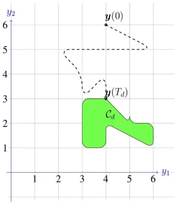
Definition 5—Confinement Control Objective Let a robot be modelled by the plant structure (1). Given a desired settling time 𝑇𝑇_𝑑𝑑 ≥0 and a desired set 𝒞𝒞_𝑑𝑑 ⊂ 𝒴𝒴 called the desired confinement set (Both:

𝑇𝑇𝑑𝑑 and 𝒞𝒞𝑑𝑑 are user specified). The confinement

control objective is defined here as:

𝑦𝑦(𝑑𝑑) ∈ 𝒞𝒞_𝑑𝑑∀𝑑𝑑 ≥ 𝑇𝑇_𝑑𝑑.

In words, the confinement control objective is achieved if the output 𝑦𝑦(𝑑𝑑) reaches at desired settling time 𝑇𝑇_𝑑𝑑 the desired confinement set 𝒞𝒞_𝑑𝑑 and it remains there for all future time𝑑𝑑 ≥ 𝑇𝑇_𝑑𝑑, see Fig. 7.

Remark 5: If the initial output 𝑦𝑦(0) starts into the desired confinement set 𝒞𝒞_𝑑𝑑, then the confinement control objective means that the output 𝑦𝑦(𝑑𝑑) will remain into the same desired confinement set 𝒞𝒞_𝑑𝑑 forever. Although it is not formally the same concept,

𝒞𝒞𝑑𝑑 may be thought-out as a kind of desired invariant

set; the latter is a concept of a proper well defined ordinary differential equation.

Remark 6: A related control objective is the so-called “reach control objective” [13] where entrances to “confinement set” are also specified.

Remark 7: Although different, the confinement control objective may be thought as a kind of

Fig. 7 “Confinement control objective” concept.

Desired confinement region 𝒞𝒞_𝑑𝑑 in green color; Trajectory output 𝑦𝑦(_𝑑𝑑) in dashed line.

uniformly ultimately boundednessof the output 𝑦𝑦. Remark 8: By proper selection of the desired confinement region 𝒞𝒞_𝑑𝑑 the usefulness of this confinement control objective arises in self-protection of robots by avoiding auto collisions (this is true for both: multi mobile robots and robot manipulators too).

6. Conclusions

In this paper a record of some nonstandard control objective concepts like velocity field control and range control with useful applications in robotics have been revisited or introduced. It opens a broad spectrum for potential control problem formulations of new high-level task robot applications like robots interaction with themselves or their environment even humans. These formulations and control design are issues of future researches.

Acknowledgments

The authors would like to thank the financial support of CONACyT under grants: 166654, 176587, and 631-295.

References

(22)

Robot Manipulators in Joint Space. London, UK: Springer.

[2] Siciliano, B., Sciavicco, L., Villani, L., and Oriolo, G. 2009. Robotics. Modelling, Planning and Control. London: Springer.

[3] Spong, M. W., Hutchinson, S., and Vidyasagar, M. 2005.

Robot Modelling and Control. Wiley.

[4] Kelly, R., and Monroy, C. 2017. “On Exotic Control Objectives in Robotics.” Presented at XIX Congreso Mexicano de Robótica COMROB2017, 8-10 de Noviembre de 2017, Mazatlán, Sin., Mexico.

[5] Khalil, H. K. 2002. Nonlinear Systems (3rd ed.). Prentice Hall.

[6] Doyle, J., Francis, B., and Tannenbaum, A. 1990.

Feedback Control Theory. Macmillan Publishing Co. [7] Kelly, R., and Monroy, C. 2014, “Desatando el nudo

gordiano del modelado de robots para fines de control: Inspiración en el cordel de Ariadna: Parte I: Rudimentos.”

AMRob Journal, Robotics: Theory and Applications 2: (4): 99-106.

[8] Li, P. Y., and Horowitz, R. 1999. “Passive Velocity Field Control of Mechanical Manipulators.” IEEE Trans. on Rob. & Auto. 15 (4): 751-63.

[9] Moreno, J., and Kelly, R. 2002. “On Manipulator Control via Velocity Fields.” In Proc. of the 15th IFAC World Congress, Barcelona, Spain.

[10] Moreno, J., and Kelly, R. 2003. “Hierarchical Velocity Field Control for Robot Manipulators.” In Proc. 2003 IEEE Int. Conf. on Rob. & Auto., Taipei, Taiwan, September 14-19, pp. 4374-9.

[11] Murray, R. M., Li, Z., and Sastry, S. S. 1994. A Mathematical Introduction to Robotic Manipulation. Boca Raton, Florida: CRC Press.

[12] Kelly, R. 2015. “Total Energy Function with Damping Assignment (TEFDA): A novel control objective in robotics.” In Proc. XVI workshop in information processing and control (RPIC), Cordoba, Argentina, DOI: 10.1109/RPIC.2015.7497057, 6-9 Oct., pp. 1-5.

[13] Helwa, M. K., and Broucke, M. E. 2015. “Flow Functions, Control Flow Functions, and the Reach Control Problem.”

Automatica 55: 108-15.

[14] Janert, P. K. 2014. “Feedback Control for Computer Systems.” O’Reilly.

[15] Alaa, M., et al. 2012. “A New Control Strategy of an Electric-Power-Assisted Steering System.” IEEE Transactions on Vehicular Technology 61 (8): 3574-89.

[16] Lee, C. M., et al. 2016. “Ride Comfort of a High-Speed Train through the Structural Upgrade of a Bogie Suspension.” Journal of Sound and Vibration 361: 99-107.

[17] Thornton, S. T., and Rex, A. 2013. Modern Physics for Scientists and Engineers (4th ed.). Cengage Learning. [18] Ericson, C. A. 2005. Hazard Analysis Techniques for

Systems Safety. Wile-Interscience.

[19] Dickinson, M. 2004. “Understanding the Mechanism of Injury and Kinetic Forces Involved in Traumatic Injuries.”

Emergency Nurse 12: 30-4.

(23)

doi: 10.17265/2159-5275/2018.02.003

Optimizing Hot Forging Process Parameters of Hollow

Parts Using Tubular and Cylindrical Workpiece:

Numerical Analysis and Experimental Validation

Angela Selau Marques, Luana De Lucca de Costa, Rafael Luciano Dalcin, Alberto Moreira Guerreiro Brito, Lirio Schaeffer and Alexandre da Silva Rocha

Faculty of Engineering, Metallurgical Department, Federal Universityof Rio Grande do Sul (UFRGS), Avenue Bento Gonçalves,

9500, Porto Alegre CEP 91509-900, Brazil

Abstract: CAE (computer aided engineering) evaluates the forging process virtually to optimize the industrial production. The numerical and experimental investigations of forging process of a hollow part are important in industrial point of view. This study has been focused on the development of a 3D elastic-plastic FEM (finite element model) of hot forging to evaluate the forming process of hollow parts. The validity of this method was verified through a laboratory experiment using aluminum alloy (AA6351) with medium geometric complexity. The distributions of effective strain, temperature, metal flow and strength were analyzed for two different initial workpieces (tubular and cylindrical). It was observed that both initial workpieces can be used to produce the final hollow part using the numerical simulation model. The results showed that the numerical analyses predict, filling cavity, calculated strength, work temperature and material flow were in agreement with the experimental results. However, some problems such as air trapping in the die causing incomplete filling could not be predicted and this problem was resolved experimentally by drilling small holes for air release in the dies.

Key words: Hot forging, FEM, hollow parts, AA6351.

1. Introduction



Economically, forged products are attractive due to

superior strength when subjected to mechanical stresses, the micro-structural homogeneity achieved

and the greater ease with which the forgings can be post-processed by automated methods [1]. The largest consumer of forged products is the automotive

industry, with an annual requirement of 58% of all world production. Recent data show that the world’s

largest producers of vehicles are China, the United States, Japan, Germany, South Korea, India, Mexico and Brazil, respectively in descending order of

production [2]. In 2014, the world produced 89.5 million cars in 2015, 91 million, and by 2020, the goal

Corresponding author: Angela Selau Marques, M.Sc., researcher, research fields: mechanical conformation and surface engineering.

is to reach 100 million cars per year [3].

The flanges are used for components such as pipes for suspension, steering and transmission systems, among others [4]. Manufacturing of flanges by means

of metal forming processes is the subject of many scientific works. Among technologies permitting

flanges forming there are the methods for full and hollow parts and for obtaining cylindrical and shaped flanges [5]. However, when a hollow part is being

forged, a machining operation is necessary to make a central hole, for instance, in this case, machining can

be eliminated if the forging process is performed from a hollow workpiece instead a massive workpiece. The hollow workpiece reduces the raw material and energy

in the forging process, which can be very significant depending on the weight, geometry, material and

batch size of the part.

(24)

Optimizing Hot Forging Process Parameters of Hollow Parts Using Tubular and Cylindrical Workpiece: Numerical Analysis and Experimental Validation

61

raw material and getting a high-quality product makes hot forging with tubular workpieces a good alternative,

mainly in the cases that long machining processes after forging are required [6]. Through numerical simulation, it is possible to find process routs for

reducing the manufacturing time and consequently, the cost [7].

In recent years, the mechanical forming industry has been experiencing a major advance in the design area due to the improvement of the numerical

simulation programs of this process [8, 9]. In the mid-1990s, most programs enabled the simulation of

the forging process for pieces with axial symmetry and others, in which the flow of material could be approximated as occurring in only two dimensions

[10]. Nowadays, it can be said that simulation programs have become an essential method for the

development and optimization of the metal forming process. Numerous commercial programs, based on different solution methods, are available in the market

[11, 12].

Within this context, the developed 3D elastic-plastic

FEM (finite element model) was used to analyze a hot closed die forging process to obtain an axial part that was used to join components in the automotive

industry using two different workpiece geometries (tubular and cylindrical). Beyond verifying the

feasibility, it will be also analyzed for possible improvements in the process and the optimization of

the process. The main objective for the use of two different geometries is obtaining the part with minimum raw material and eliminating experimental

work that would be necessary without a previous simulation.

2. Material Data

The material used to make the workpieces was a

commercially available AA6351 aluminum alloy. The chemical components of AA6351 are listed in Table 1.

It was showed in flow curves determined experimentally that not only strain but also strain rate and temperature have a great influence on the flow

properties of AA6351 [13]. According to Fig. 1, the flow stress increases as the temperature decreases and

the strain rate increases.

However, to facilitate insertion of material flow curves into numerical simulation software is necessary

that they can be represented by a mathematical equation, considering the model of Hansel-Spittel, in

Eq. (1). Table 2 gives the values of the optimized Hansel-Spittel parameter.

σ . e T_._ε _. ₍₁₎

The mechanical and thermal properties of the AA6351 aluminum alloy material are listed in Table 3.

Table 1 Chemical components of AA6351.

Al Si Fe Mg Mn Ti Zn Cu

97.07 0.42 0.29 0.82 0.24 0.013 0.01 0.18

(25)

Table 2 Optimized parameters of the Hansel-Spittel model [12].

Parameters Hansel-Spittel

(MPa) 303.5

m1 -0.0043

m2 0.103

m3 0.057

T (°C) 400

Table 3 Mechanical and thermal properties of the AA6351.

Parameters Values

Density (kg/m3) 2,600

Poisson’sratio 0.33

Young modulus (GPa) 70-80 (T dependent)

Specific heat (J/(g-K)) 0.89

Thermal conductivity (W/(m-K)) 176

Heat transfer coefficient (blank-tools) (W/(m2K)) 12.5 (150 MPa)

Table 4 Mechanical and thermal properties of the H13.

Parameters Values

Density (kg/m3) 7,690

Poisson’sratio 0.33

Young modulus (GPa) 210 (T dependent)

Specific heat (J/(g-K)) 0.460

Thermal conductivity (W/(m-K)) 24.7

The commercially available H13 tool steel was used

to make the dies. The mechanical and thermal properties of the H13 material are listed in Table 4.

3. Numerical Modeling

The geometry of the final part is shown in Fig. 2. It

was obtained through the 3D modeling of the part developed in the SolidWorks® software. The use of this system allowed a series of automations with

regard to the modeling of the part, workpieces and dies.

Fig. 3 shows the main dimensions (mm) of the study part. The walls of the piece were designed with angle of 7. A higher angle was chosen to avoid the

probability of adhesion of the piece to the tool.

The dimensions of the tube were: height of 35.5

mm, width of 41.5 mm and concentric hole of 12 mm in diameter. The dimensions of the cylindrical workpiece were: height of 32 mm and width of 41.5

mm. It was possible to estimate the dimensions of the initial workpiece by the volume conservation law,

considering the volumes of the final part, the flash and

the flash land.

The designs of the flash land and the parting line were required to develop the dies project. Fig. 4 shows

a cross-sectional view of the upper and lower dies, the air out channel, the guide pin and a simulated piece

representation.

The software Simufact® was used to evaluate the die filling and the manufacturing of parts within

dimensional tolerances. Furthermore, the parameters that were involved in the process were also analyzed,

such as the workpiece and die geometry, forging strength, temperature and friction. The finite element method was chosen to analyze the forging process.

Due to the geometry of the part, a 3D simulation was used, the results of which are more reliable and fit

better to the hot forging process. These considerations are indicated in the literature by the software manufacturer and others studies [8].

(26)

Optimizing Hot Forging Process Parameters of Hollow Parts Using Tubular and Cylindrical Workpiece: Numerical Analysis and Experimental Validation

63

Fig. 2 (a) The 3D representation of the part to be forged; and (b) Cross-sectional view.

Fig. 3 The main dimensions of the final part.

Fig. 4 Design of the upper and lower dies.

this stage, the type of process is defined, for example,

if it would be a hot or cold forging process, and the number of dies which would be used in the simulation.

The thermal and mechanical properties of the AA6351 and H13 aluminum alloy are described in

Tables 3 and 4 and these were inserted into the

Simufact Software database. The true stress-strain

curves of the AA6351 at various temperatures are input into the preprocessor of Simufact. Forming in the form of table, showed in Table 1. The material of

the workpieces is defined as a homogeneous and isotropic elastic-plastic body. The tools are considered

(27)

Friction and contact heat conduction exist at the interfaces between the blank and the tools. Hence, the

Coulomb friction model is employed, and the friction coefficients are assumed to be constant during analysis.

The mesh size, type and number of elements will be informed by the software, and the data influence

directly on the results presented by the simulation [8]. The simulations were performed with two types of mesh, 2D and 3D, and it was determined that the best

mesh to be used is 3D, since it had satisfactory results. Thus, a mesh of 1 mm was used, the type of element

was hexahedral and the number of elements created was 15.484. Fig. 5 shows this mesh.

The parameters of the process used in the

simulation are very important for reliable results and are shown in Fig. 6.

4. Experimental Forging Process

The same parameters of the simulation were used in

order to compare the results obtained in the numerical simulation and the experiments performed. The

hydraulic press with capacity of 6.000 kN and tool velocity of 3.4 mm/s was used in the experimental process. The parameter configurations for the operation

of the hydraulic press were done through a system called Siemens HMI. This interface system allows one

to set all the parameters of the hydraulic press and change them, if it is necessary. The dies were connected to the press with appropriate clamps to

avoid the occurrence of relative movements between the dies during the forging process. The tools had

guide pins to prevent shifting during the process. They

were heated by conduction temperature to 300 °C. The workpieces were heated to a temperature of

400 °C in an electric furnace. In the process sequence, these workpieces were dipped in synthetic lubricant solution in order to obtain a lubricating film

surrounding them. The dies were sprayed with the same synthetic lubricant solution to obtain a better

lubricating surface.