World Scientific Publishing Co. Pte. Ltd. 5 Toh Tuck Link, Singapore 596224
USA office: 27 Warren Street, Suite 401-402, Hackensack, NJ 07601 UK office: 57 Shelton Street, Covent Garden, London WC2H 9HE
Library of Congress Cataloging-in-Publication Data Names: Simovici, Dan A., author.
Title: Mathematical analysis for machine learning and data mining / by Dan Simovici (University of Massachusetts, Boston, USA).
Description: [Hackensack?] New Jersey : World Scientific, [2018] | Includes bibliographical references and index.
Identifiers: LCCN 2018008584 | ISBN 9789813229686 (hc : alk. paper) Subjects: LCSH: Machine learning--Mathematics. | Data mining--Mathematics. Classification: LCC Q325.5 .S57 2018 | DDC 006.3/101515--dc23
LC record available at https://lccn.loc.gov/2018008584
British Library Cataloguing-in-Publication Data
A catalogue record for this book is available from the British Library.
Copyright © 2018 by World Scientific Publishing Co. Pte. Ltd.
All rights reserved. This book, or parts thereof, may not be reproduced in any form or by any means, electronic or mechanical, including photocopying, recording or any information storage and retrieval system now known or to be invented, without written permission from the publisher.
For photocopying of material in this volume, please pay a copying fee through the Copyright Clearance Center, Inc., 222 Rosewood Drive, Danvers, MA 01923, USA. In this case permission to photocopy is not required from the publisher.
For any available supplementary material, please visit
http://www.worldscientific.com/worldscibooks/10.1142/10702#t=suppl
Desk Editors: V. Vishnu Mohan/Steven Patt Typeset by Stallion Press
Making mathematics accessible to the educated layman, while keeping high scientific standards, has always been considered a treacherous navigation between the Scylla of professional contempt and the Charybdis of public misunderstanding.
Mathematical Analysis can be loosely described as is the area of mathemat-ics whose main object is the study of function and of their behaviour with respect to limits. The term “function” refers to a broad collection of gen-eralizations of real functions of real arguments, to functionals, operators, measures, etc.
There are several well-developed areas in mathematical analysis that present a special interest for machine learning: topology (with various fla-vors: point-set topology, combinatorial and algebraic topology), functional analysis on normed and inner product spaces (including Banach and Hilbert spaces), convex analysis, optimization, etc. Moreover, disciplines like mea-sure and integration theory which play a vital role in statistics, the other pillar of machine learning are absent from the education of a computer scientists. We aim to contribute to closing this gap, which is a serious handicap for people interested in research.
The machine learning and data mining literature is vast and embraces a diversity of approaches, from informal to sophisticated mathematical pre-sentations. However, the necessary mathematical background needed for approaching research topics is usually presented in a terse and unmotivated manner, or is simply absent. This volume contains knowledge that comple-ments the usual presentations in machine learning and provides motivations (through its application chapters that discuss optimization, iterative algo-rithms, neural networks, regression, and support vector machines) for the study of mathematical aspects.
Each chapter ends with suggestions for further reading. Over 600 ex-ercises and supplements are included; they form an integral part of the material. Some of the exercises are in reality supplemental material. For these, we include solutions. The mathematical background required for
making the best use of this volume consists in the typical sequence calcu-lus — linear algebra — discrete mathematics, as it is taught to Computer Science students in US universities.
Special thanks are due to the librarians of the Joseph Healy Library at the University of Massachusetts Boston whose diligence was essential in completing this project. I also wish to acknowledge the helpfulness and competent assistance of Steve Patt and D. Rajesh Babu of World Scientific. Lastly, I wish to thank my wife, Doina, a steady source of strength and loving support.
Dan A. Simovici Boston and Brookline
Preface vii
Part I. Set-Theoretical and Algebraic Preliminaries
1
1. Preliminaries 3
1.1 Introduction . . . 3
1.2 Sets and Collections . . . 4
1.3 Relations and Functions . . . 8
1.4 Sequences and Collections of Sets . . . 16
1.5 Partially Ordered Sets . . . 18
1.6 Closure and Interior Systems . . . 28
1.7 Algebras andσ-Algebras of Sets . . . 34
1.8 Dissimilarity and Metrics . . . 43
1.9 Elementary Combinatorics . . . 47
Exercises and Supplements . . . 54
Bibliographical Comments . . . 64
2. Linear Spaces 65 2.1 Introduction . . . 65
2.2 Linear Spaces and Linear Independence . . . 65
2.3 Linear Operators and Functionals . . . 74
2.4 Linear Spaces with Inner Products . . . 85
2.5 Seminorms and Norms . . . 88
2.6 Linear Functionals in Inner Product Spaces . . . 107
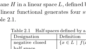
2.7 Hyperplanes . . . 110
Exercises and Supplements . . . 113
Bibliographical Comments . . . 116
3. Algebra of Convex Sets 117
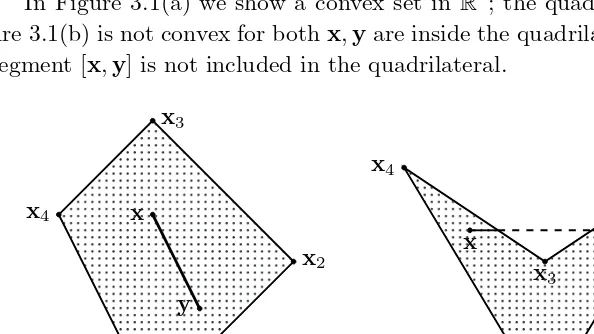
3.1 Introduction . . . 117
3.2 Convex Sets and Affine Subspaces . . . 117
3.3 Operations on Convex Sets . . . 129
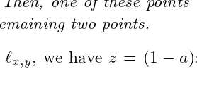
3.4 Cones . . . 130
3.5 Extreme Points . . . 132
3.6 Balanced and Absorbing Sets . . . 138
3.7 Polytopes and Polyhedra . . . 142
Exercises and Supplements . . . 150
Bibliographical Comments . . . 158
Part II. Topology
159
4. Topology 161 4.1 Introduction . . . 1614.2 Topologies . . . 162
4.3 Closure and Interior Operators in Topological Spaces . . . 166
4.4 Neighborhoods . . . 174
4.5 Bases . . . 180
4.6 Compactness . . . 189
4.7 Separation Hierarchy . . . 193
4.8 Locally Compact Spaces . . . 197
4.9 Limits of Functions . . . 201
4.10 Nets . . . 204
4.11 Continuous Functions . . . 210
4.12 Homeomorphisms . . . 218
4.13 Connected Topological Spaces . . . 222
4.14 Products of Topological Spaces . . . 225
4.15 Semicontinuous Functions . . . 230
4.16 The Epigraph and the Hypograph of a Function . . . 237
Exercises and Supplements . . . 239
Bibliographical Comments . . . 253
5. Metric Space Topologies 255 5.1 Introduction . . . 255
5.2 Sequences in Metric Spaces . . . 260
5.4 Continuity of Functions between Metric Spaces . . . 264
5.5 Separation Properties of Metric Spaces . . . 270
5.6 Completeness of Metric Spaces . . . 275
5.7 Pointwise and Uniform Convergence . . . 283
5.8 The Stone-Weierstrass Theorem . . . 286
5.9 Totally Bounded Metric Spaces . . . 291
5.10 Contractions and Fixed Points . . . 295
5.11 The Hausdorff Metric Hyperspace of Compact Subsets . . . 300
5.12 The Topological Space (R,O) . . . 303
5.13 Series and Schauder Bases . . . 307
5.14 Equicontinuity . . . 315
Exercises and Supplements . . . 318
Bibliographical Comments . . . 327
6. Topological Linear Spaces 329 6.1 Introduction . . . 329
6.2 Topologies of Linear Spaces . . . 329
6.3 Topologies on Inner Product Spaces . . . 337
6.4 Locally Convex Linear Spaces . . . 338
6.5 Continuous Linear Operators . . . 340
6.6 Linear Operators on Normed Linear Spaces . . . 341
6.7 Topological Aspects of Convex Sets . . . 348
6.8 The Relative Interior . . . 351
6.9 Separation of Convex Sets . . . 356
6.10 Theorems of Alternatives . . . 366
6.11 The Contingent Cone . . . 370
6.12 Extreme Points and Krein-Milman Theorem . . . 373
Exercises and Supplements . . . 375
Bibliographical Comments . . . 381
Part III. Measure and Integration
383
7. Measurable Spaces and Measures 385 7.1 Introduction . . . 3857.2 Measurable Spaces . . . 385
7.3 Borel Sets . . . 388
7.5 Measures and Measure Spaces . . . 398
7.6 Outer Measures . . . 417
7.7 The Lebesgue Measure onRn . . . 427
7.8 Measures on Topological Spaces . . . 450
7.9 Measures in Metric Spaces . . . 453
7.10 Signed and Complex Measures . . . 456
7.11 Probability Spaces . . . 464
Exercises and Supplements . . . 470
Bibliographical Comments . . . 484
8. Integration 485 8.1 Introduction . . . 485
8.2 The Lebesgue Integral . . . 485
8.2.1 The Integral of Simple Measurable Functions . . . 486
8.2.2 The Integral of Non-negative Measurable Functions . . . 491
8.2.3 The Integral of Real-Valued Measurable Functions . . . 500
8.2.4 The Integral of Complex-Valued Measurable Functions . . . 505
8.3 The Dominated Convergence Theorem . . . 508
8.4 Functions of Bounded Variation . . . 512
8.5 Riemann Integral vs. Lebesgue Integral . . . 517
8.6 The Radon-Nikodym Theorem . . . 525
8.7 Integration on Products of Measure Spaces . . . 533
8.8 The Riesz-Markov-Kakutani Theorem . . . 540
8.9 Integration Relative to Signed Measures and Complex Measures . . . 547
8.10 Indefinite Integral of a Function . . . 549
8.11 Convergence in Measure . . . 551
8.12 Lp andLp Spaces . . . 556
8.13 Fourier Transforms of Measures . . . 565
8.14 Lebesgue-Stieltjes Measures and Integrals . . . 569
8.15 Distributions of Random Variables . . . 572
8.16 Random Vectors . . . 577
Exercises and Supplements . . . 582
Part IV. Functional Analysis and Convexity
595
9. Banach Spaces 597
9.1 Introduction . . . 597
9.2 Banach Spaces — Examples . . . 597
9.3 Linear Operators on Banach Spaces . . . 603
9.4 Compact Operators . . . 610
9.5 Duals of Normed Linear Spaces . . . 612
9.6 Spectra of Linear Operators on Banach Spaces . . . 616
Exercises and Supplements . . . 619
Bibliographical Comments . . . 623
10. Differentiability of Functions Defined on Normed Spaces 625 10.1 Introduction . . . 625
10.2 The Fr´echet and Gˆateaux Differentiation . . . 625
10.3 Taylor’s Formula . . . 649
10.4 The Inverse Function Theorem inRn . . . 658
10.5 Normal and Tangent Subspaces for Surfaces in Rn . . . . 663
Exercises and Supplements . . . 666
Bibliographical Comments . . . 675
11. Hilbert Spaces 677 11.1 Introduction . . . 677
11.2 Hilbert Spaces — Examples . . . 677
11.3 Classes of Linear Operators in Hilbert Spaces . . . 679
11.3.1 Self-Adjoint Operators . . . 681
11.3.2 Normal and Unitary Operators . . . 683
11.3.3 Projection Operators . . . 684
11.4 Orthonormal Sets in Hilbert Spaces . . . 686
11.5 The Dual Space of a Hilbert Space . . . 703
11.6 Weak Convergence . . . 704
11.7 Spectra of Linear Operators on Hilbert Spaces . . . 707
11.8 Functions of Positive and Negative Type . . . 712
11.9 Reproducing Kernel Hilbert Spaces . . . 722
11.10 Positive Operators in Hilbert Spaces . . . 733
Exercises and Supplements . . . 736
12. Convex Functions 747
12.1 Introduction . . . 747
12.2 Convex Functions — Basics . . . 748
12.3 Constructing Convex Functions . . . 756
12.4 Extrema of Convex Functions . . . 759
12.5 Differentiability and Convexity . . . 760
12.6 Quasi-Convex and Pseudo-Convex Functions . . . 770
12.7 Convexity and Inequalities . . . 775
12.8 Subgradients . . . 780
Exercises and Supplements . . . 793
Bibliographical Comments . . . 815
Part V. Applications
817
13. Optimization 819 13.1 Introduction . . . 81913.2 Local Extrema, Ascent and Descent Directions . . . 819
13.3 General Optimization Problems . . . 826
13.4 Optimization without Differentiability . . . 827
13.5 Optimization with Differentiability . . . 831
13.6 Duality . . . 843
13.7 Strong Duality . . . 849
Exercises and Supplements . . . 854
Bibliographical Comments . . . 863
14. Iterative Algorithms 865 14.1 Introduction . . . 865
14.2 Newton’s Method . . . 865
14.3 The Secant Method . . . 869
14.4 Newton’s Method in Banach Spaces . . . 871
14.5 Conjugate Gradient Method . . . 874
14.6 Gradient Descent Algorithm . . . 879
14.7 Stochastic Gradient Descent . . . 882
Exercises and Supplements . . . 884
15. Neural Networks 893
15.1 Introduction . . . 893
15.2 Neurons . . . 893
15.3 Neural Networks . . . 895
15.4 Neural Networks as Universal Approximators . . . 896
15.5 Weight Adjustment by Back Propagation . . . 899
Exercises and Supplements . . . 902
Bibliographical Comments . . . 907
16. Regression 909 16.1 Introduction . . . 909
16.2 Linear Regression . . . 909
16.3 A Statistical Model of Linear Regression . . . 912
16.4 Logistic Regression . . . 914
16.5 Ridge Regression . . . 916
16.6 Lasso Regression and Regularization . . . 917
Exercises and Supplements . . . 920
Bibliographical Comments . . . 924
17. Support Vector Machines 925 17.1 Introduction . . . 925
17.2 Linearly Separable Data Sets . . . 925
17.3 Soft Support Vector Machines . . . 930
17.4 Non-linear Support Vector Machines . . . 933
17.5 Perceptrons . . . 939
Exercises and Supplements . . . 941
Bibliographical Comments . . . 947
Bibliography 949
Preliminaries
1.1 Introduction
This introductory chapter contains a mix of preliminary results and nota-tions that we use in further chapters, ranging from set theory, and combi-natorics to metric spaces.
The membership of x in a set S is denoted by x ∈ S; if x is not a member of the setS, we writex∈S.
Throughout this book, we use standardized notations for certain impor-tant sets of numbers:
C the set of complex numbers R the set of real numbers
R0 the set of non-negative real numbers
R>0 the set of positive real numbers
R0 the set of non-positive real numbers
R<0 the set of negative real numbers
ˆ
C the setC∪ {∞} ˆ
R the setR∪ {−∞,+∞} Rˆ0 the setR0∪ {+∞} ˆ
R0 the setR0∪ {−∞} Rˆ>0 the setR<>0∪ {+∞} Q the set of rational numbers I the set of irrational numbers
Z the set of integers N the set of natural numbers
The usual order of real numbers is extended to the set ˆRby−∞< x <
+∞for everyx∈R. Addition and multiplication are extended by
x+∞=∞+x= +∞, and, x− ∞=−∞+x=−∞,
for everyx∈R. Also, ifx= 0 we assume that
x· ∞=∞ ·x=
+∞ ifx >0, −∞ ifx <0,
and
x·(−∞) = (−∞)·x=
−∞ ifx >0, ∞ ifx <0.
Additionally, we assume that 0·∞=∞·0 = 0 and 0·(−∞) = (−∞)·0 = 0. Note that∞ − ∞,−∞+∞are undefined.
Division is extended byx/∞=x/− ∞= 0 for everyx∈R.
The set of complex numbersCis extended by adding a single “infinity” element ∞. The sum∞+∞isnot definedin the complex case.
IfS is a finite set, we denote by|S|the number of elements ofS.
1.2 Sets and Collections
We assume that the reader is familiar with elementary set operations: union, intersection, difference, etc., and with their properties. The empty set is denoted by∅.
We give, without proof, several properties of union and intersection of sets:
(1) S∪(T∪U) = (S∪T)∪U (associativity of union), (2) S∪T =T∪S (commutativity of union),
(3) S∪S=S (idempotency of union), (4) S∪ ∅=S,
(5) S∩(T∩U) = (S∩T)∩U (associativity of intersection), (6) S∩T =T∩S (commutativity of intersection),
(7) S∩S=S (idempotency of intersection), (8) S∩ ∅=∅,
for all setsS, T, U.
The associativity of union and intersection allows us to denote unam-biguously the union of three setsS, T, U byS∪T∪U and the intersection of three setsS, T, U byS∩T∩U.
Definition 1.1. The setsS andT aredisjoint ifS∩T =∅.
Sets may contain other sets as elements. For example, the set
C={∅,{0},{0,1},{0,2},{1,2,3}}
IfC andD are two collections, we say thatC isincluded inD, or that C is asubcollection ofD, if every member ofCis a member of D. This is denoted by C⊆D.
Two collectionsC andD are equal if we have both C⊆Dand D⊆C. This is denoted by C=D.
Definition 1.2. LetCbe a collection of sets. Theunion ofC, denoted by
C, is the set defined by
C={x | x∈Sfor some S∈C}.
IfCis anon-emptycollection, itsintersectionis the setCgiven by
C={x | x∈S for everyS∈C}.
If C = {S, T}, we have x ∈ C if and only if x ∈ S or x ∈ T and
x∈Cif and only ifx∈S andy∈T. The union and the intersection of this two-set collection are denoted by S∪T andS∩T and are referred to as the union and the intersection ofS andT, respectively.
The difference of two setsS, T is denoted byS−T. WhenT is a subset of Swe write T forS−T, and we refer to the setT as thecomplementof
T with respect to S or simply thecomplement ofT.
The relationship between set difference and set union and intersection is well-known: for every set S and non-empty collectionCof sets, we have
S−C={S−C | C∈C}andS−C={S−C | C∈C}.
For any sets S, T, U, we have
S−(T∪U) = (S−T)∩(S−U) andS−(T∩U) = (S−T)∪(S−U).
With the notation previously introduced for the complement of a set, the above equalities become:
T∪U =T∩U andT ∩U =T∪U .
For any setsT,U,V, we have
(U∪V)∩T = (U∩T)∪(V ∩T) and (U∩V)∪T = (U∪T)∩(V ∪T).
Note that ifCandDare two collections such thatC⊆D, then
C⊆Dand D⊆C.
∅ =S for the empty collection of subsets of S. This is consistent with the fact that∅ ⊆CimpliesC⊆S.
Thesymmetric difference of sets denoted by ⊕is defined by U⊕V = (U−V)∪(V −U) for all setsU, V.
We leave to the reader to verify that for all setsU, V, T we have (i) U⊕U =∅;
(ii) U⊕V =V ⊕T;
(iii) (U⊕V)⊕T =U⊕(V ⊕T).
The next theorem allows us to introduce a type of set collection of fundamental importance.
Theorem 1.1. Let {{x, y},{x}}and{{u, v},{u}}be two collections such that {{x, y},{x}}={{u, v},{u}}. Then, we have x=uandy=v.
Proof. Suppose that{{x, y},{x}}={{u, v},{u}}.
If x = y, the collection {{x, y},{x}} consists of a single set, {x}, so the collection {{u, v},{u}} also consists of a single set. This means that
{u, v} = {u}, which implies u = v. Therefore, x = u, which gives the desired conclusion because we also havey=v.
If x = y, then neither (x, y) nor (u, v) are singletons. However, they both contain exactly one singleton, namely {x} and {u}, respectively, so
x=u. They also contain the equal sets {x, y} and {u, v}, which must be equal. Since v∈ {x, y} andv=u=x, we conclude thatv=y.
Definition 1.3. An ordered pairis a collection of sets{{x, y},{x}}.
Theorem 1.1 implies that for an ordered pair{{x, y},{x}},xandyare uniquely determined. This justifies the following definition.
Definition 1.4. Let {{x, y},{x}}be an ordered pair. Thenx isthe first component of pandy isthe second component ofp.
From now on, an ordered pair{{x, y},{x}}is denoted by (x, y). If both
x, y ∈S, we refer to (x, y) as anordered pair on the set S.
Definition 1.5. LetX, Y be two sets. Theirproductis the setX×Y that consists of all pairs of the form (x, y), wherex∈X andy∈Y.
The set product is often referred to as theCartesian product of sets.
Example 1.1. LetX ={a, b, c}and letY ={1,2}. The Cartesian product
X×Y is given by
Definition 1.6. LetC and D be two collections of sets such that C =
D
. D is a refinementof Cif, for everyD ∈D, there existsC ∈C such that D⊆C.
This is denoted byC⊑D.
Example 1.2. Consider the collection C = {(a,∞) | a ∈ R} and D =
{(a, b) | a, b∈R, a < b}. It is clear thatC=D=R.
Since we have (a, b) ⊆ (a,∞) for every a, b ∈ R such that a < b, it follows thatDis a refinement ofC.
Definition 1.7. A collection of setsC is hereditary ifU ∈C and W ⊆U
impliesW ∈C.
Example 1.3. LetS be a set. The collection of subsets ofS, denoted by P(S), is a hereditary collection of sets since a subset of a subset T ofS is itself a subset ofS.
The set of subsets of S that contain k elements is denoted byPk(S).
Clearly, for every set S, we haveP0(S) = {∅} because there is only one
subset ofS that contains 0 elements, namely the empty set. The set of all finite subsets of a set S is denoted by Pfin(S). It is clear that Pfin(S) =
k∈NPk(S).
Example 1.4. If S = {a, b, c}, then P(S) consists of the following eight sets: ∅,{a},{b},{c},{a, b},{a, c},{b, c},{a, b, c}. For the empty set, we haveP(∅) ={∅}.
Definition 1.8. LetCbe a collection of sets and letU be a set. Thetrace of the collection Con the set U is the collectionCU ={U∩C | C∈C}.
We conclude this presentation of collections of sets with two more op-erations on collections of sets.
Definition 1.9. Let C and D be two collections of sets. The collections C∨D,C∧D, andC−D are given by
C∨D={C∪D | C∈CandD∈D},
C∧D={C∩D | C∈CandD∈D},
C−D={C−D | C∈CandD∈D}.
Example 1.5. LetCandDbe the collections of sets defined by C={{x},{y, z},{x, y},{x, y, z}},
We have
C∨D={{x, y},{y, z},{x, y, z},{u, y, z},{u, x, y, z}},
C∧D={∅,{x},{y},{x, y},{y, z}},
C−D={∅,{x},{z},{x, z}},
D−C={∅,{u},{x},{y},{u, z},{u, y, z}}.
Unlike “∪” and “∩”, the operations “∨” and “∧” between collections of sets are not idempotent. Indeed, we have, for example,
D∨D={{y},{x, y},{u, y, z},{u, x, y, z}} =D.
The trace CK of a collectionConKcan be written asCK =C∧ {K}.
We conclude this section by introducing a special type of collection of subsets of a set.
Definition 1.10. A partition of a non-empty set S is a collection π of non-empty subsets of S that are pairwise disjoint and whose union equals
S.
The members ofπare referred to as theblocksof the partitionπ. The collection of partitions of a setS is denoted byPART(S). A parti-tion is finite if it has a finite number of blocks. The set of finite partiparti-tions of Sis denoted by PARTfin(S).
Ifπ ∈PART(S) then a subset T of S is π-saturated if it is a union of blocks ofπ.
Example 1.6. Let π = {{1,3},{4},{2,5,6}} be a partition of S =
{1,2,3,4,5,6}. The set {1,3,4} is π-saturated because it is the union of blocks {1,3}and 4.
1.3 Relations and Functions
Definition 1.11. LetX, Y be two sets. Arelation on X, Y is a subsetρ
of the set product X×Y.
IfX =Y =S we refer toρas arelation onS.
The relationρonS is:
• reflexive if (x, x)∈ρfor everyx∈S;
• irreflexive if (x, x)∈ρfor everyx∈S;
• antisymmetric if (x, y) ∈ ρ and (y, x) ∈ ρ imply x = y for all
x, y∈S;
• transitiveif (x, y)∈ρand (y, z)∈ρimply (x, z)∈ρfor allx, y, z∈ S.
Denote byREFL(S),SYMM(S),ANTISYMM(S) andTRAN(S) the sets of reflexive relations, the set of symmetric relations, the set of antisymmetric, and the set of transitive relations on S, respectively.
A partial order on S is a relation ρ that belongs to REFL(S) ∩ ANTISYMM(S)∩TRAN(S), that is, a relation that is reflexive, symmetric and transitive.
Example 1.7. Let δ be the relation that consists of those pairs (p, q) of natural numbers such that q =pk for some natural number k. We have (p, q)∈δifpevenly dividesq. Since (p, p)∈δfor everypit is clear thatδ
is symmetric.
Suppose that we have both (p, q)∈δ and (q, p)∈δ. Thenq=pk and
p=qh. If eitherp or q is 0, then the other number is clearly 0. Assume that neither pnorqis 0. Then 1 =hk, which impliesh=k= 1, sop=q, which proves that δis antisymmetric.
Finally, if (p, q),(q, r)∈δ, we haveq=pkandr=qhfor somek, h∈N, which impliesr=p(hk), so (p, r)∈δ, which shows thatδis transitive.
Example 1.8. Define the relation λ on R as the set of all ordered pairs (x, y) such that y = x+t, where t is a non-negative number. We have (x, x)∈λbecausex=x+ 0 for everyx∈R. If (x, y)∈λand (y, x)∈λwe havey=x+tandx=y+sfor two non-negative numberst, s, which implies 0 = t+s, so t = s = 0. This means that x= y, soλ is antisymmetric. Finally, if (x, y),(y, z) ∈ λ, we have y = x+u and z = y +v for two non-negative numbers u, v, which impliesz=x+u+v, so (x, z)∈λ.
In current mathematical practice, we often writexρyinstead on (x, y)∈
ρ, where ρ is a relation of S and x, y ∈ S. Thus, we write pδq and xλy
instead on (p, q)∈δand (x, y)∈λ. Furthermore, we shall use the standard notations “|” and “” forδ andλ, that is, we shall writep | qandxy
ifpdividesqandxis less or equal toy. This alternative way to denote the fact that (x, y) belongs toρis known as theinfix notation.
Example 1.9. LetP(S) be the set of subsets ofS. It is easy to verify that the inclusion between subsets “⊆” is a partial order relation on P(S). If
Functions are special relation that enjoy the property described in the next definition.
Definition 1.12. LetX, Y be two sets. A function (or a mapping) from X toY is a relationf onX, Y such that (x, y),(x, y′)∈f impliesy=y′.
In other words, the first component of a pair (x, y) ∈ f determines uniquely the second component of the pair. We denote the second compo-nent of a pair (x, y) ∈f by f(x) and say, occasionally, that f maps x to y.
Iff is a function fromX toY we writef :X −→Y.
Definition 1.13. LetX, Y be two sets and letf :X −→Y. Thedomainoff is the set
Dom(f) ={x∈X | y=f(x) for somey∈Y}.
Therange off is the set
Ran(f) ={y∈Y | y=f(x) for somex∈X}.
Definition 1.14. LetX be a set, Y ={0,1} and let Lbe a subset of S. Thecharacteristic functionis the function 1L:S−→ {0,1}defined by:
1L(x) =
1 ifx∈L,
0 otherwise
forx∈S.
Theindicator functionofLis the function IL:S−→rrˆ defined by
IL(x) =
0 ifx∈L, ∞ otherwise forx∈S.
It is easy to see that:
1P∩Q(x) = 1P(x)·1Q(x),
1P∪Q(x) = 1P(x) + 1Q(x)−1P(x)·1Q(x),
1P¯(x) = 1−1P(x),
for everyP, Q⊆S andx∈S.
Proof. Let (x, z1),(x, z2)∈gf. There existy1, y2∈Y such that
y1=f(x), y2=f(x), g(y1) =z1, andg(y2) =z2.
The first two equalities imply y1 =y2; the last two yieldz1=z2, so gf is
indeed a function.
Note that the composition of the functionf andghas been denoted in Theorem 1.2 by gf rather than the relation productf g. This manner of denoting the function composition is applied throughout this book.
Definition 1.15. Let X, Y be two sets and let f : X −→ Y. If U is a subset ofX, the restrictionof f to U is the function g :U −→Y defined byg(u) =f(u) foru∈U.
The restriction off toU is denoted byf ↿U.
Example 1.10. Letf be the function defined byf(x) =|x|forx∈R. Its restriction toR<0 is given byf ↿R<0 (x) =−x.
Definition 1.16. A functionf :X −→Y is:
(i) injectiveorone-to-oneiff(x1) =f(x2) impliesx1=x2forx1, x2∈
Dom(f);
(ii) surjectiveor ontoifRan(f) =Y; (iii) totalif Dom(f) =X.
Iff is both injective and surjective, then it is abijective function.
Theorem 1.3. A function f : X −→ Y is injective if and only if there exists a functiong:Y −→X such thatg(f(x)) =xfor everyx∈Dom(f).
Proof. Suppose that f is an injective function. For x ∈ Dom(f) and
y =f(x) define g(y) = x. Note that g is well defined for if y =f(x1) = f(x2) thenx1=x2due to the injectivity off. It follows immediately that g(f(x)) =xforx∈Dom(f).
Conversely, suppose that there exists a functiong:Y −→X such that
g(f(x)) =xfor everyx∈Dom(f). Iff(x1) =f(x2), thenx1=g(f(x1)) = g(f(x2)) =x2, which proves thatf is indeed injective.
The functiong whose existence is established by Theorem 1.3 is said to be the left inverse of f. Thus, a function f : X −→Y is injective if and only if it has a left inverse.
The Axiom of Choice: LetC={Ci | i∈I}be a collection
of non-empty sets indexed by a setI. There exists a function
φ:I−→C
(known as achoice function) such thatφ(i)∈Ci
for eachi∈I.
Theorem 1.4. A function f : X −→ Y is surjective if and only if there exists a function h:X −→Y such thatf(h(y)) =y for everyy∈Y.
Proof. Suppose thatf is a surjective function. The collection{f−1(y) | y ∈Y} indexed byY consists of non-empty sets. By the Axiom of Choice there exists a choice function for this collection, that is a functionh:Y −→
y∈Yf−1(y) such thath(y)∈f−1(y), orf(h(y)) =yfory∈Y.
Conversely, suppose that there exists a functionh:X −→Y such that
f(h(y)) =y for every y ∈Y. Then, f(x) =y fory =h(y), which shows
that f is surjective.
The functionhwhose existence is established by Theorem 1.4 is said to be theright inverseoff. Thus, a function has a right inverse if and only if it is surjective.
Corollary 1.1. A function f :X −→X is a bijection if and only if there exists a functionk:X −→X that is both a left inverse and a right inverse of f.
Proof. This statement follows from Theorems 1.3 and 1.4.
Indeed, iff is a bijection, there exists a left inverseg :X −→X such that g(f(x)) =xand a right inverseh: X −→ X such thatf(h(x)) =x
for everyx∈Y. Sinceh(x)∈X we haveg(f(h(x))) =h(x), which implies
g(x) =h(x) becausef(h(x)) =xforx∈X. This yieldsg=h.
The relationship between the subsets of a set and characteristic func-tions defined on that set is discussed next.
Theorem 1.5. There is a bijection Ψ : P(S)−→ (S −→ {0,1})between the set of subsets ofS and the set of characteristic functions defined onS.
Proof. ForP ∈P(S) define Ψ(P) = 1P. The mapping Ψ is one-to-one.
Indeed, assume that 1P = 1Q, whereP, Q∈P(S). We have x∈P if and
only if 1P(x) = 1, which is equivalent to 1Q(x) = 1. This happens if and
only ifx∈Q; hence,P =Qso Ψ is one-to-one.
set Tf; hence, Ψ(Tf) = f which shows that the mapping Ψ is also onto;
hence, it is a bijection.
Definition 1.17. A setS isindexedbe a setI if there exists a surjection
f :I−→S. In this case we refer toI as an index set.
If S is indexed by the function f : I −→ S we write the element f(i) just assi, if there is no risk of confusion.
Definition 1.18. A sequence of length n on a set X is a function x :
{0,1, . . . , n−1} −→X.
At times we will use the same term to designate a function x :
{1, . . . , n} −→X.
Sequences are denoted by bold letters. Ifxis a sequence of lengthnwe refer tox(i) as theithofx; this element ofX is denoted usually byxi. We
specify a sequencexof lengthnby writing
x= (x0, x1, . . . , xn−1).
The set of sequence of lengthnon a setX is denoted bySeqn(X).
Note that an ordered pair (x, y)∈X×Y can be regarded as a sequence
p of length 2 onX∪Y such thatp0=xand p1 =y. This point of view
allows an immediate generalization of set products.
Definition 1.19. Aninfinite sequence, or, simply asequenceon a setX is a function x:N−→X. The set of infinite sequences onX is denoted by
Seq(X).
Definition 1.20. Let S0, . . . , Sn−1 ben sets. Ann-tupleonS0, . . . , Sn−1
is a function t : {0, . . . , n−1} −→ S0∪ · · ·Sn−1 such that t(i) ∈ Si for
0in−1. Then-tuplet is denoted by (t(0), . . . , t(n−1)).
The set of all n-tuples onS0, . . . , Sn−1 is referred to as the Cartesian
product ofS0, . . . , Sn−1 and is denoted byS0× · · · ×Sn−1.
The Cartesian product of a finite number of sets can be generalized for arbitrary families of sets. Let S = {Si | i ∈ I} be a collection of sets indexed by the setI. The Cartesian product ofSis the set of all functions of the form s: I −→ Ssuch that s(i)∈ Si for everyi ∈ I. This set is denoted by i∈ISi.1
The notion ofprojectionis closely associated to Cartesian products. 1This constructions is implicitly using the axiom of choice that implies the existence of functionss:I−→
Definition 1.21. LetS={Si | i∈I} be a collection of sets indexed by the setI. Thejth projection(forj∈I) is the mappingpj:
i∈ISi−→Sj
defined by pj(s) =s(j) forj∈I.
Definition 1.22. LetX, Y be two sets and letf :X−→Y be a function. IfU ⊆Dom(f), theimageofU underf is the set
f(U) ={y∈Y | y=f(u) for someu∈X}.
IfT ⊆Y, thepre-imageofT underf is the setf−1(T) =
{x∈X | f(x)∈
Y}.
Theorem 1.6. Let X, Y be two sets and let f :X −→Y be a function. If V ⊆Y, thenX−f−1(V) =f−1(Y
−V).
Proof. Ifx∈X−f−1(V), we havef(x)∈V, so f(x)∈Y −V, which
means that x∈f−1(Y
−V). Therefore,X−f−1(V)
⊆f−1(Y −V). Conversely, suppose that x ∈ f−1(Y −V), so f(x) ∈ V, hence x ∈ f−1(V), which means thatx
∈X−f−1(V), which completes the proof.
Theorem 1.7. Let f :X−→Y be a function. IfU, V ⊆Dom(f)we have f(U∪V) =f(U)∪f(V)andf(U∩V)⊆f(U)∩f(V).
IfS, T⊆Ran(f), thenf−1(S∪T) =f−1(S)∪f−1(T)andf−1(S∩T) = f−1(S)
∩f−1(T).
Proof. This statement is a direct consequence of Definition 1.22.
Theorem 1.8. Let f : X −→ Y be a function. We have U ⊆f−1(f(U))
for every subsetU of X andf(f−1(V))
⊆V for every subset V of Y.
Proof. Letx∈u. Sincef(x)∈f(U), it follows that u∈f−1(f(U)), so U ⊆f−1(f(U)).
If y ∈f(f−1(V)) there exists x
∈f−1(V) such that y =f(x). Since f(x)∈V, it follows thaty∈V, sof(f−1(V))
⊆V.
Theorem 1.9. Let X, Y be two sets and let f : X −→ Y be a function. If U ⊆X, then Ran(f)−f(U)⊆f(Dom(f)−U). If f is injective, then
Ran(f)−f(U) =f(Dom(f)−U).
Proof. Lety∈Ran(f)−f(U). Then, there existsx∈Dom(f) such that
y=f(x); however, sincey ∈f(U), there is nox1∈U such thaty=f(x1).
Thus, x∈Dom(f)−U and we have the desired inclusion.
Suppose now that f is injective and let y ∈ f(Dom(f)−U). Then,
y ∈f(U) for otherwise, we would havey=f(x1) for some x1∈U, x=x1
(because x∈U andx1 ∈U), and this would contradict the injectivity of f. Thus,y∈Ran(f)−f(U) and we obtain the desired equality.
Corollary 1.2. Let f:X −→X be a injection. We havef(U) =f(U)for every subsetU of X.
Proof. Since f is a bijection, we have Ran(f) = X, so X −f(U) =
f(X−U) by Theorem 1.9, which amounts tof(U) =f(U).
Theorem 1.10. Let f : X −→ Y be a function. If V, W ⊆ Y, then f−1(V −W) = f−1(V)−f−1(W). Furthermore, if C = {Yi | i ∈ I} is
a collection of subsets of Y we have f−1
i∈ICi =
i∈If−1(Ci) and f−1i∈ICi =
i∈If−1(Ci).
Proof. Letx∈f−1(V −W). We havef(x)∈V andf(x)∈W.
There-fore,x∈f−1(V) andx
∈f−1(W), sox
∈f−1(V)
−f−1(W). Conversely,
suppose that x∈f−1(V)
−f−1(U), that is, x
∈f−1(V) andx
∈f−1(U).
This means that f(x)∈ V and f(x)∈U, so f(x)∈ V −U, which yields
f(x)∈ V −U. Thus, x∈ f−1(V
−U), which concludes the proof of the first equality.
Let now x ∈ f−1
i∈ICi . This implies f(x) ∈ Ci for every i ∈ I,
so x ∈ f−1(Ci) for each i
∈ I. Therefore, x ∈ i∈If−1(Ci), so f−1
i∈ICi ⊆
i∈If−1(Ci).
Conversely, letx∈i∈If−1(Ci). We havex
∈f−1(Ci) for everyi ∈I, sof(x)∈Cifori∈I. Therefore,f(x)∈i∈ICi, hencex∈f−1
i∈ICi .
We leave to the reader to prove the third equality of the theorem.
Definition 1.23. Let X, Y be two finite non-empty and disjoint sets and let ρ be a relation, ρ ⊆X ×Y. A perfect matching for ρ is an injective mapping f :X −→Y such that ify=f(x), then (x, y)∈ρ.
Note that a perfect matching of ρis an injective mappingf such that
f ⊆ρ.
For a subsetAofX define the setρ[A] as
ρ[A] ={y∈Y | (x, y)∈ρfor some x∈A}.
Theorem 1.11. (Hall’s Perfect Matching Theorem)LetX, Y be two finite non-empty and disjoint sets and letρbe a relation,ρ⊆X×Y. There exists a perfect matching for ρif and only if for every A∈P(X) we have
Proof. The proof is by induction on |X|. If |X| = 1, the statement is immediate.
Suppose that the statement holds for|X|nand consider a setXwith
|X|=n+ 1. We need to consider two cases: either |ρ[A]|>|A| for every subsetA ofX, or there exists a subsetA ofX such that|ρ[A]|=|A|.
In the first case, since|ρ[{x}]|>1 there existsy∈Y such that (x, y)∈ρ. LetX′=X− {x},Y′=Y− {y}, and letρ′=ρ∩(X′×Y′). Note that
for every B ⊆X′ we have|ρ′[B]| |B|+ 1 because for every subset Aof
X we have|ρ[A| |A|+ 1 and deleting a single elementy from ρ[A] still leaves at least|A|elements in this set. By the inductive hypothesis, there exists a perfect matchingf′forρ′. This matching extends to a matchingf
forρby definingf(x) =y.
In the second case, letAbe a proper subset ofX such that|ρ[A]|=|A|. Define the sets X′, Y′, X′′, Y′′as
X′=A, X′′=X−A,
Y′=ρ[A], Y′′=Y −ρ[A]
and consider the relationsρ′=ρ∩(X′×Y′), andρ′′=ρ∩(X′′×Y′′). We
shall prove that there are perfect matchings f′ andf′′ for the relations ρ′
and ρ′′. A perfect matching forρwill be given byf′∪f′′.
SinceAis a proper subset ofX we have both|A|nand|X−A|n. For any subsetB ofAwe haveρ′[B] =ρ[B], soρ′ satisfies the condition of the theorem and a perfect matchingf′ forρ′ exists.
Suppose that there existsC⊆X′′ such that|ρ′′[C]|<|C|. This would imply |ρ[C∪A]| < |C∪A| because ρ[C∪A] = ρ′′[C]∪ρ[A], which is
impossible. Thus, ρ′′ also satisfies the condition of the theorem and a
perfect matching exists for ρ′′.
1.4 Sequences and Collections of Sets
Definition 1.24. A sequence of setsS= (S0, S1, . . . , Sn, . . .) isexpanding
ifi < j impliesSi⊆Sj for everyi, j∈N.
If i < j implies Sj ⊆ Si for every i, j ∈ N, then we say that S is a contracting sequence of sets.
A sequence of sets ismonotoneif it is expanding or contracting.
Definition 1.25. LetSbe an infinite sequence of subsets of a setS, where
The set ∞i=0∞j=iSj is referred to as the lower limit of S; the set
∞
i=0 ∞
j=iSjis theupper limitofS. These two sets are denoted by lim infS
and lim supS, respectively.
If x ∈ lim infS, then there exists i such that x ∈ ∞j=iSj; in other
words, xbelongs to all but finitely many setsSi.
Ifx∈lim supS, then, for everyi there existsjisuch that such that
x∈Sj; in this casexbelongs to infinitely many sets of the sequence. Clearly, we have lim infS⊆lim supS.
Definition 1.26. A sequence of setsSisconvergentif lim infS= lim supS. In this case the set L= lim infS= lim supSis said to be the limitof the sequenceSand is denoted by limS.
Example 1.11. Every expanding sequence of sets is convergent. Indeed, sinceSis expanding we have∞j=iSj=Si. Therefore, lim infS=∞i=0Si. On the other hand,∞j=iSj⊆∞i=0Siand, therefore, lim supS⊆lim infS. This shows that lim infS= lim supS, that is,Sis convergent.
A similar argument can be used to show thatSis convergent whenSis contracting.
In this chapter we will use the notion of set countability discussed, for example, in [56].
Definition 1.27. LetCbe a collection of subsets of a setS. The collection Cσ consists of all countable unions of members ofC.
The collection Cδ consists of all countable intersections of members
of C,
Cσ= ⎧ ⎨ ⎩
n0
Cn | Cn∈C
⎫ ⎬
⎭ andCδ = ⎧ ⎨ ⎩
n0
Cn | Cn∈C
⎫ ⎬ ⎭.
Observe that by takingCn=C∈Cforn0 it follows thatC⊆Cσand
C⊆Cδ. Furthermore, if C,C′ are two collections of sets such that C⊆C′,
thenCσ ⊆C′σand C′δ⊆Cδ.
Theorem 1.12. For any collection of subsetsCof a setSwe have(Cσ)σ=
Cσ and(Cδ)δ =Cδ.
The operationsσandδcan be applied iteratively. We denote sequences of applications of these operations by subscripts adorning the affected col-lection. The order of application coincides with the order of these symbols in the subscript. For example (C)σδσ means ((Cσ)δ)σ. Thus, Theorem 1.12
can be restated as the equalities Cσσ=Cσ andCδδ =Cδ.
Observe that ifC= (C0, C1, . . .) is a sequence of sets, then lim supC= ∞
i=0 ∞
j=iCj ∈ Cσδ and lim infC = ∞i=0 ∞
j=iCj belongs to Cδσ, where
C={Cn | n∈N}.
1.5 Partially Ordered Sets
Ifρis a partial order onS, we refer to the pair (S, ρ) as apartially ordered setor as a poset.
Astrict partial order, ora strict orderonS, is a relationρ⊆S×Sthat is irreflexive and transitive.
Note that ifρis a partial order onS, the relation
ρ1=ρ− {(x, x) | x∈S}
is a strict partial order onS.
From now on we shall denote by “” a generic partial order on a setS; thus, a generic partially ordered set is denoted by (S,).
Example 1.12. Let δ = {(m, n) | m, n ∈ N, n = km for somek ∈ N}. Since n= 1nit follows that (n, n)∈δ for everyn∈N, soδ is a reflexive relation. Suppose that (m, n)∈δand (n, m)∈δ, son=mk andm=nh
for some k, h ∈ N. This implies n(1−kh) = 0. If n = 0, it follows that m = 0. If n = 0 we have kh = 1, which means that k = h = 1 because k, h∈N, so again,m =n. Thus, δ is antisymmetric. Finally, if (m, n),(n, p)∈δwe haven=rmandp=snfor somer, s∈N, sop=srm, which implies (m, p)∈δ. This shows thatδis also transitive and, therefore, it is a partial order relation onN.
Example 1.13. Letπ, σ be two partitions inPART(S). We define πσ
if each blockC ofσis a π-saturated set.
It is clear that “” is a reflexive relation. Suppose that π σ and
σ τ, where π, σ, τ ∈PARTfin(S). Then each block D of τ is a union of
blocks of σ, and each block of σ is a union of blocks of π. Thus, D is a union of blocks ofπand, therefore, πτ.
Since no block of a partition can be a subset of another block of the same partition, it follows that each block of σ coincides with a block ofπ, that is σ=π.
Definition 1.28. Let (S,) be a poset and let K ⊆S. The set of upper boundsof the setK is the setKs=
{y∈S | xy for everyx∈K}. The set of lower bounds of the set K is the set Ki = {y ∈ S | y xfor everyx∈K}.
IfKs=∅, we say that the setK isbounded above. Similarly, ifKi=∅,
we say thatK isbounded below. IfK is both bounded above and bounded below we will refer to K as abounded set.
IfKs=
∅(Ki=
∅), thenK is said to be unbounded above (below).
Theorem 1.13. Let (S,)be a poset and let U and V be two subsets of S. If U ⊆V, then we have Vi⊆Ui andVs⊆Us.
Also, for every subset T of S, we haveT ⊆(Ts)i andT
⊆(Ti)s.
Proof. The argument for both statements of the theorem amounts to a
direct application of Definition 1.28.
Note that for every subsetT of a posetS, we have both
Ti= ((Ti)s)i (1.1)
and
Ts= ((Ts)i)s. (1.2)
Indeed, since T ⊆ (Ti)s, by the first part of Theorem 1.13, we have
((Ts)i)s
⊆ Ts. By the second part of the same theorem applied to Ts,
we have the reverse inclusionTs
⊆((Ts)i)s, which yieldsTs= ((Ts)i)s.
Theorem 1.14. For any subset K of a poset (S, ρ), the setsK∩Ks and K∩Ki contain at most one element.
Proof. Suppose that y1, y2 ∈ K∩Ks. Since y1 ∈ K and y2 ∈ Ks, we
have (y1, y2) ∈ ρ. Reversing the roles of y1 and y2 (that is, considering
now thaty2∈K andy1∈Ks), we obtain (y2, y1)∈ρ. Therefore, we may
conclude thaty1=y2because of the antisymmetry of the relationρ, which
shows that K∩Kscontains at most one element.
A similar argument can be used for the second part of the proposition;
we leave it to the reader.
Definition 1.29. Let (S,) be a poset. Theleast (greatest) elementof the subsetKofSis the unique element of the setK∩Ki(K
∩Ks, respectively)
IfKis unbounded above, then it is clear thatKhas no greatest element. Similarly, if Kis unbounded below, thenK has no least element.
Applying Definition 1.29 to the setS, theleast (greatest) elementof the poset (S,) is an elementaofS such thatax(xa, respectively) for allx∈S.
It is clear that if a poset has a least element u, then u is the unique minimal element of that poset. A similar statement holds for the greatest and the maximal elements.
Definition 1.30. The subsetKof the poset (S,) has aleast upper bound uifKs
∩(Ks)i= {u}.
K has thegreatest lower boundv ifKi
∩(Ki)s= {v}.
We note that a set can have at most one least upper bound and at most one greatest lower bound. Indeed, we have seen above that for any set U
the setU∩Uimay contain an element or be empty. Applying this remark
to the setKs, it follows that the setKs∩(Ks)i may contain at most one
element, which shows thatK may have at most one least upper bound. A similar argument can be made for the greatest lower bound.
If the set K has a least upper bound, we denote it by supK. The greatest lower bound of a set will be denoted by infK. These notations come from the Latin terms supremumand infimumused alternatively for the least upper bound and the greatest lower bound, respectively.
Lemma 1.1. Let U, V be two subsets of a poset (S,). If U ⊆ V then Vs
⊆Usand Vi ⊆Ui.
Proof. This statement follows immediately from the definitions of the sets of upper bounds and lower bounds, respectively.
Theorem 1.15. Let(S,)be a poset and letK, Lbe two subsets ofS such that K⊆L.
If supK and supLexist, then supKsupL; if infK andinfLexist, then infLinfK.
Proof. By Lemma 1.1 we have Ls
⊆ Ks and Li
⊆ Ki. By the same Lemma, we have: (Ks)i⊆(Ls)i and (Ki)s⊆(Li)s.
Let a= supK and b = supL. Since{a} =Ks
∩(Ks)i and (Ks)i ⊆
(Ls)i, it follows thata
∈(Ls)i. Sinceb
∈Ls, this implies ab.
Ifc= infK andd= infL, taking into account that{c}=Ki∩(Ki)s,
we havec∈(Li)sbecauseKi
∩(Ki)s
⊆(Li)s. Sinced
∈Liwe havedc.
Example 1.14. A two-element subset{m, n}of the poset (N, δ) introduced in Example 1.12 has both an infimum and a supremum. Indeed, letpbe the least common multiple ofmand n. Since (n, p),(m, p)∈δ, it is clear that
pis an upper bound of the set{m, n}. On the other hand, ifkis an upper bound of{m, n}, thenkis a multiple of bothmandn. In this case,kmust also be a multiple of pbecause otherwise we could writek =pq+rwith 0< r < pby dividingkbyp. This would implyr=k−pq; hence,rwould be a multiple of both mand nbecause both k and phave this property. However, this would contradict the fact that p is the least multiple that
m and n share! This shows that the least common multiple of m and n
coincides with the supremum of the set{m, n}. Similarly, inf{m, n}equals the greatest common divisormandn.
Example 1.15. Let π, σ be two partitions in PART(S). It is easy to see that the collection θ={B∩C | B ∈π, C ∈σ, B∩C =∅} is a partition of S; furthermore, ifτ is a partition ofS such thatπτ andστ, then each block E of τ is both a π-saturated set and a σ-saturated set, and, therefore a θ-saturated set. This shows thatτ = inf{π, σ}.
The partition will be denoted byπ∧σ.
Definition 1.31. Aminimal elementof a poset (S,) is an elementx∈S
such that {x}i =
{x}. A maximal element of (S,) is an element y ∈ S
such that{y}s= {y}.
In other words, x is a minimal element of the poset (S,) if there is no element less than or equal to xother than itself; similarly,xis maximal if there is no element greater than or equal toxother than itself.
For the poset (R,), it is possible to give more specific descriptions of the supremum and infimum of a subset when they exist.
Theorem 1.16. If T ⊆ R, then u = supT if and only if u is an upper bound of T and, for everyǫ >0, there ist∈T such thatu−ǫ < tu.
The number v is infT if and only if v is a lower bound of T and, for every ǫ >0, there is t∈T such that vt < v+ǫ.
Proof. We prove only the first part of the theorem; the argument for the second part is similar and is left to the reader.
Suppose that u= supT; that is,{u}=Ts∪(Ts)i. Sinceu∈Ts, it is
upper bound forT, and in this caseucannot be a lower bound for the set of upper bounds ofT. Therefore, no suchǫmay exist.
Conversely, suppose thatuis an upper bound ofT and for everyǫ >0, there is t ∈T such that u−ǫ < tu. Suppose that u does not belong to (Ks)i. This means that there is another upper bound u′ of T such
that u′ < u. Choosing ǫ = u−u′, we would have no t ∈ T such that
u−ǫ = u′ < t u because this would prevent u′ from being an upper
bound of T. This impliesu∈(Ks)i, sou= supT.
Theorem 1.17. In the extended poset of real numbers( ˆR,)every subset has a supremum and an infimum.
Proof. If a set is bounded then the existence of the supremum and in-fimum is established by the Completeness Axiom. Suppose that a subset
S of ˆRhas no upper bound in R. Thenx∞, so∞ is an upper bound of S in ˆR. Moreover ∞ is the unique upper bound of S, so supS =∞. Similarly, if S has no lower bound inR, then infS =−∞in ˆR.
The definitions of infimum and supremum of the empty set in ( ˆR,) are
sup∅=−∞and inf∅=∞,
in order to remain consistent with Theorem 1.15. A very important axiom for the setRis given next.
The Completeness Axiom forR: IfTis a non-empty subset ofRthat is bounded above, thenT has a supremum.
A statement equivalent to the Completeness Axiom forRfollows.
Theorem 1.18. If T is a non-empty subset of R that is bounded below, then T has an infimum.
Proof. Note that the set Ti is not empty. If s
∈ Ti and t
∈ T, we have st, so the setTi is bounded above. By the Completeness Axiom v= supTi exists and
{v}= (Ti)s
∩((Ti)s)i= (Ti)s
∩Ti by equality (1.1).
Thus, v= infT.
We leave to the reader to prove that Theorem 1.18 implies the Com-pleteness Axiom for R.
Theorem 1.19. (Dedekind’s Theorem)LetU andV be non-empty sub-sets of Rsuch thatU ∪V =Randx∈U, y∈V imply x < y. Then, there existsa∈Rsuch that ifx > a, thenx∈V, and if x < a, thenx∈U.
Proof. Observe thatU =∅andV ⊆Us. SinceV =∅, it means thatU is
bounded above, so by the Completeness Axiom supU exists. Leta= supU. Clearly,u≤afor everyu∈U. SinceV ⊆Us, it also follows thatav for
everyv∈V.
If x > a, then x ∈ V because otherwise we would have x ∈ U since
U ∪V =Rand this would implyxa. Similarly, ifx < a, thenx∈U.
Using the previously introduced notations, Dedekind’s theorem can be stated as follows: ifU andV are non-empty subsets ofRsuch thatU∪V = R,Us
⊆V,Vi
⊆U, then there existsasuch that{a}s
⊆V and{a}i ⊆U. One can prove that Dedekind’s theorem implies the Completeness Ax-iom. Indeed, let T be a non-empty subset of R that is bounded above. ThereforeV =Ts
=∅. Note thatU = (Ts)i
=∅andU∪V =R. Moreover,
Us = ((Ts)i)s =Ts=V andVi = (Ts)i =U. Therefore, by Dedekind’s
theorem, there is a∈R such that{a}s
⊆V =Ts and {a}i
⊆U = (Ts)i.
Note thata∈ {a}s∩ {a}i⊆Ts∩(Ts)i, which proves thata= supT.
By adding the symbols +∞and −∞to the setR, one obtains the set ˆ
R. The partial orderdefined onRcan now be extended to ˆRby−∞x
and x+∞for everyx∈R.
Note that, in the poset ( ˆR,), the sets Ti and Ts are non-empty for
everyT ∈P( ˆR) because −∞ ∈Ti and +
∞ ∈Tsfor any subsetT of ˆR.
Theorem 1.20. For every set T ⊆ Rˆ, both supT and infT exist in the poset ( ˆR,).
Proof. We present the argument for supT. If supT exists in (R,), then it is clear that the same number is supT in ( ˆR,).
Assume now that supT does not exist in (R,). By the Completeness Axiom forR, this means that the setT does not have an upper bound in (R,). Therefore, the set of upper bounds ofT in ( ˆT ,) isTsˆ={+∞}.
It follows immediately that in this case supT = +∞in ( ˆR,).
Theorem 1.21. Let I be a partially ordered set and let {xi | i∈I} be a subset of Rˆ indexed by I. Fori∈I let Si ={xj | j ∈I andi j}. We have
Proof. Note that ifih, thenSh ⊆Si fori, h∈I. As we saw earlier, each setSihas both an infimumyiand a supremumziin the poset ( ˆR,). It is clear that ifih, thenyiyhzhzi. We claim that
sup{yi | i∈I}inf{zh | h∈I}.
Indeed, since thenyi zhfor alli, hsuch thatih, we haveyi inf{zh | h∈I} for alli∈I. Therefore,
sup{yi | i∈I}inf{zh | h∈I},
which can be written as
sup infSiinf supSi.
LetS be a set and let f :S −→Rˆ. The image ofS underf is the set
f(S) ={f(x) | x∈S}. Sincef(S)⊆R, supˆ f(S) exists. Furthermore, if there exists u∈S such that f(u) = supf(S), then we say that f attains its supremumatu. This is not always the case as the next example shows.
Example 1.16. Letf : (0,1)−→Rˆ be defined byf(x) = 1−1x. It is clear that supf((0,1)) =∞. However, there is nou∈(0,1) such thatf(u) =∞, so f does not attain its supremum on (0,1).
LetX, Y be two sets and letf :X×Y −→Rˆ be a function. We have
sup
x∈X
inf
y∈Yf(x, y)yinf∈Yxsup∈Xf(x, y). (1.4)
Indeed, note that infy∈Y f(x, y)f(x, y) for everyx∈X andy ∈Y by
the definition of the infimum. Note that the left member of the inequality depends only on x. The last inequality implies supx∈Xinfy∈Yf(x, y)
supx∈Xf(x, y), by the monotonicity of sup and now the current left member
is a lower bound of the set {z = supx∈Xf(x, y) | y ∈ Y}. This implies
immediately the inequality (1.4).
If instead of inequality (1.4) the functionf satisfies the equality:
sup
x∈Xyinf∈Yf(x, y) = infy∈Yxsup∈Xf(x, y), (1.5)
then the common value of both sides is asaddle valueforf.
Since infy∈Y f(x, y) is a function h(x) of x and supx∈Xf(x, y) is a
If both supx∈Xh(x) and infy∈Y g(y) are attained, that is, there are x0∈X and y0∈Y such that
h(x0) = sup x∈X
h(x) = sup
x∈X
inf
y∈Yf(x, y), g(y0) = inf
y∈Yg(y) = infy∈Yxsup∈Xf(x, y),
we have
h(x0) = sup x∈X
inf
y∈Yf(x, y)
= inf
y∈Yxsup∈Xf(x, y)
(because of the existence of the saddle value) = inf
y∈Yg(y) =g(y0).
Therefore,
g(y0) = sup x∈X
f(x, y0) =f(x0, y0) = inf
y∈Yf(x0, y) =h(x0),
and
f(x, y0)f(x0, y0)f(x0, y).
The pair (x0, y0) that satisfies the inequalities
f(x, y0)f(x0, y0)f(x0, y)
is referred to as asaddle pointforf.
Conversely, if there exists a saddle point (x0, y0) such thatf(x, y0) f(x0, y0)f(x0, y), thenf :X×Y −→Rhas a saddle value. Indeed, in
this case we
sup
x∈X
f(x, y0)f(x0, y0) inf
y∈Yf(x0, y),
hence
inf
y∈Yxsup∈Xf(x, y)xsup∈Xf(x, y0)f(x0, y0)yinf∈Yf(x0, y)xsup∈Xyinf∈Yf(x, y).
Since a saddle value exists, these inequalities become equalities and we have a saddle value.
Definition 1.32. Let (S,) be a poset. A chain of (S,) is a subset T
of S such that for everyx, y∈T such that x=y we have eitherx < y or
Example 1.17. The set of real numbers equipped with the usual partial order (R,) is a chain since, for every x, y ∈R, we have eitherxy or
yx.
Theorem 1.22. If {Ui | i ∈I} is a chain of the poset (CHAINS(S),⊆) (that is, a chain of chains of (S,)), then {Ui | i∈I} is itself a chain of (S,) (that is, a member of(CHAINS(S),⊆)).
Proof. Letx, y∈{Ui | i∈I}. There arei, j∈I such thatx∈Uiand
y ∈Uj and we have either Ui ⊆Uj or Uj ⊆Ui. In the first case, we have either xi xj or xj xi because both xand y belong to the chain Uj. The same conclusion can be reached in the second case when both xand
y belong to the chainUi. So, in any case,xand y are comparable, which
proves that{Ui | i∈I}is a chain of (S,).
A statement equivalent to a fundamental principle of set theory known as the Axiom of Choice is Zorn’s lemma stated below.
Zorn’s Lemma: If every chain of a poset (S,) has an upper bound, thenS has a maximal element.
Theorem 1.23. The following three statements are equivalent for a poset (S,):
(i) If every chain of (S,)has an upper bound, thenS has a maximal element (Zorn’s Lemma).
(ii) If every chain of (S,) has a least upper bound, then S has a maximal element.
(iii) S contains a chain that is maximal with respect to set inclusion (Hausdorff2 maximality principle).
Proof. (i) implies (ii)is immediate.
(ii) implies (iii): Let (CHAINS(S),⊆) be the poset of chains ofSordered by set inclusion. Every chain {Ui | i ∈ I} of the poset (CHAINS(S),⊆) has a least upper bound {Ui | i ∈ I} in the poset (CHAINS(S),⊆).
2Felix Hausdorff was born on November 8th, 1868 in Breslau in Prussia, (now Germany) and died on January 26th, 1942 in Bonn, Germany. Hausdorff is one of the founders of modern topology and set theory, and has major contributions in measure theory, and functional analysis.
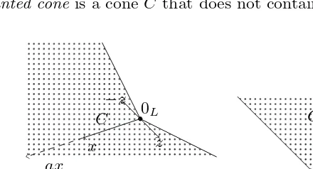
![Fig. 3.6Triangulation of a 2-simplex S[x1, x2, x3].](https://thumb-ap.123doks.com/thumbv2/123dok/3935579.1878999/164.595.83.329.166.327/fig-triangulation-of-a-simplex-s-x-x.webp)