Stability Analysis on Effect of Jawa Bali Power System Loading Using Developed State Space Program - repository civitas UGM

(1)

Stability Analysis on Effect of Jawa-Bali Power System Loading

Using Developed State Space Program

Avrin Nur Widiastuti

Electrical Dept., Engineering Fac. Gadjah Mada University, e-mail:avrin@.ugm.ac.id, pinkpisan@yahoo.com

Abstract – This study develops a program to generate linearized state space representation of the power systems. The two-axis model of synchronous generator and the IEEE type I model of exciter are used to represent dynamic behaviors of the generating units. The developed program can accommodate an actual structure of the power systems with some numbers of generating units and the AC buses. Furthermore, the effect of loading on Jawa Bali Power System is studied. The real loads at a particular bus are increased continuously. At each step, the initial conditions of the state variables are computed, after running the load flow, and linearization of the equations is done. The matrix A is formed, and its eigenvalues are checked for stability. If unstable, the program will identify the states associated with the unstable eigenvalues of matrix A using the participation factor method. From the result of the developed program, we see that the dynamic performance of the system is change as the given operating conditions change, the real part of eigenvalue is bigger so that the system is more unstable. All of the unstable modes are associated with state variable

δ

of machine 1, 6 and 8, and also the state variable

E

_qof machine 5. With this study, it helps Indonesian utility to predict the maximum loading of the powers system within stability region and for control design, thereafter.

I.

INTRODUCTION

The analysis of dynamic stability can be performed by deriving the linearized state space model of the system in the following form :

ݔ ൌ ܣݔ ൅ ܤݑሶ (1)

where the matrices A and B also depend on the given operating conditions. The eigenvalues of the state matrix A determine the small-signal stability around the given operating point. The eigenvalues analysis can be used not only for the determination of the stability regions, but also for the design of the controllers [1].

In this study we develop the program to generate linearized state space model of multimachine power systems that is necessary for the study of both small signal stability analysis, voltage stability and for control design, thereafter.

II.

POWERSYSTEMDYNAMICMODEL

The overall power system representation in this research includes models for the following components:

• synchronous generator and the associated excitation systems

• AC transmission network including static fixed-impedance, loads For system stability studies concerning electromechanical oscillation, it is appropriate to neglect the transmission network and the machine stator transients [2]. The dynamics of synchronous generator rotor circuits and excitation systems are represented by the sets of differential equations. The result is that the complete system model consists of a large number of non-linear ordinary differential and algebraic equations. We can describe complex power system as our plant which consists of generators, transmission network as depicted in Fig. 1. It is noted that there can be a number of generators in the system.

Network including load

generator generator

Figure 1 Complex power system

A.

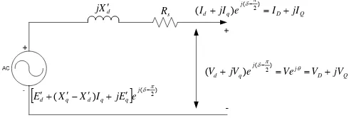
Synchronous Generator Model

We will use a simplified generator model with two axes adopted from [3] as show in Fig. 2

d

X j ′

s

R

[

]

)

2 (

) (

π δ − ′ + ′ − ′ +

′ j

q q d q

d X X I jE e

E

Q D j q

d jI e I jI

I + ₎ (−2)= +

(

π δ

Q D j j q

d jV e Ve V jV

V + − = θ= +

π δ )

2 (

) (

Figure 2 Two-axis synchronous machine model Defines :

X d is the d-axis transient synchronous reactance X q′ is the q-axis transient synchronous reactance Rs is the armature resistance

I d is the d-axis current refer to the mach. ref. frame I q is the q-axis current refer to the mach. ref. frame I D is the d-axis current refer to the netw. ref. frame IQ is the q-axis current refer to the netw. ref. Frame

τq′0 is the q-axis transient open circuit time constant

τd′0 is the d-axis transient open circuit time constant X d is the d-axis synchronous reactance

X q is the q-axis synchronous reactance

δ is the angular position of the rotor

ω is the angular velocity of rotor Eq′ is the q-axis transient voltage Ed′ is the d-axis transient voltage E fd is the DC field voltage

ωs is the rated value of an angular velocity of rotor TM is the mechanical torque applied

Te is the electromagnetic torque developed TD is the damping torque component D is the damping factor

H is the inertia constant

From the above figure, the stator algebraic equation can be written as :

) 2 (

)

)(

(

π δ

θ

₊

_′

₊

j −

q d d s

j

_R

_j

_X

_I

_jI

_e

Ve

0 ]

)

(

[

′

+

′

−

′

+

′

( 2)

=

−

π δ

j q q d q

d

X

I

j

E

e

E

(2)

fd

E

is the exciter voltage

R

V

is the regulator voltage

F

R

is the stabilizer voltage

A

K

is the voltage regulator gain

A

τ

is the voltage regulator time constant

E

K

is the exciter gain

E

τ

is the exciter time constant

F

K

is the regulator stabilizing circuit gain

F

τ

is the regulator stabilizing circ time constant

EX

S

is the rotating exctr saturation at ceiling voltage

EX

A

is the saturation const for rotating exciters

EX

(2)

Multiplying eq. (2) by

) 2 (δ−π

−j

e

_{and equating the real and the imaginary}

parts, we obtain :

In addition, the dynamic behaviors of the rotor motion and the rotor circuits can be describing using the following differential equations :

s

B.

Excitation System

In order to improve the damping characteristics of the synchronous generator, supplementary excitation controls have been widely employed. In this study, we use the IEEE type I exciter as shown in Figure 3

⎥

Figure 3 Block diagram of the IEEE type I excitation control

From the block diagram above, we have three following equations :

E

C.

AC Transmission System

The network characteristics in this study described in the form of power balance. The network can consist of many electrical buses and branches depending on the system of interest. Some of the buses connect to the

generators and called generator buses. The rest of the buses which are not connected to generating units called as load bus.

• Generator buses

The two equations representing real and reactive power balance for each generator bus are given below. For real power balance,

)

For reactive power balance,

)

For the load buses, we have equations for both real and reactive power also. For real power balance,

0

For reactive power balance,

0 P

and

Q

_Liand are voltage dependence loads. In this study, loads are assumed as constant power type.

D.

Linearized State Space Model of Power Systems

• Linearized State Space Model

The behavior of a dynamic system, such as a power system, may be described by a set of n first order nonlinear ordinary differential equations of the following form :

If equations (20) is linearized around the given operating states and inputs

)

,

(

x

₀

u

₀ , then the linearized state equation can be written as follows :

u

Reference [4] shows that the linearized state space model will be usefull for design controller that can be applied in the system.

• Eigenvalue and Stability

After the linearized state space representation of the system is obtained such as eq.21, we can see the eigenvalues of the system by inspection of matrix

A

, which reveal the stability of system.

A negative real eigenvalue represents a decaying mode. The larger its magnitude, the faster the decay (system stable), while a positive real eigenvalue represent instability [5,6,7,8,9].

(3)

Figure 4 An algorithm to generate linearized state space model

In addition, the damping ratio can be computed as :

2

_ω

σ

ζ

+

−

=

(24)

• Participation Factor

Participation factor analysis aids in the identification of how each state variable is reflected on a given mode or eigenvalue [3]. Participation factor

ki

p

is defined as

∑

=

n

k ki ik ik ki ki

w

v

w

v

p

1

(25)

Where

ki

p

is the participation factor relating the

k

thstate variable to the

i

th

eigenvalue

ki

w

and

v

_kiare the

k

th entries in the left and right eigenvector

associated with the

i

th eigenvalue.

A further normalization can be done by making the largest of the participation factors equal to unity.

The formulation of the state equations involves the development of linearized equation about an operating point and elimination of all non state and non input variables. However, the need to allow for the representation of extensive transmission network, loads and excitation system, makes the process very complex. Therefore, the formulation of the state equations requires a systematic procedure for treating the wide range of devices.

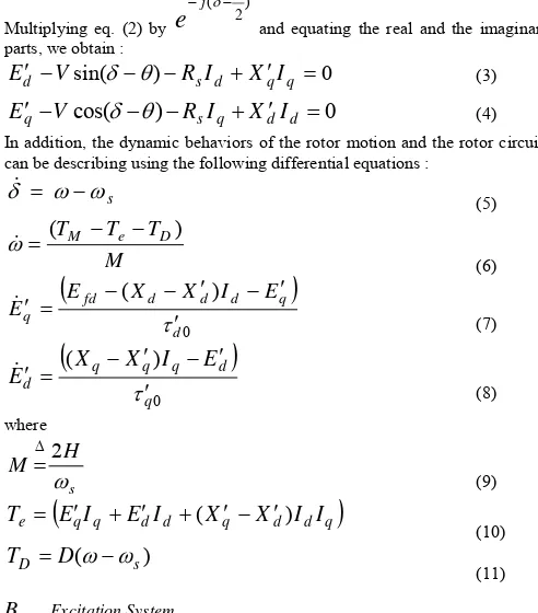
Figure 5 Flowchart on effect of loading of power system

III.

SIMULATION AND RESULT

A.

State Space Model Generation Algorithm

The first step of the program is read input data from all components. After that the program will run load flow to calculate the operating point of the network. From operating point, program will continue to calculate initial condition all variables in generator. Then program will calculate the matrix for each equation and do many calculations based on the algorithm to develop state model [10]. The flow chart is in Fig. 4.

B.

Effect of loading on 500 KVJawa Bali power system

In this study the effect of loading on the small signal stability of the system is studied using the developed program. The real or reactive loads at a particular bus/buses are increased continuously. At each step, the initial conditions of the state variables are computed, after running the load flow, and linearization of the equations is done. The matrix Asys is formed, and its eigenvalues are checked for stability. If unstable, the program will identify the states associated with the unstable eigenvalues of matrix Asys using the participation factor method. The flow chart of this study is in Figure 5.

The developed program is applied for 500 KV Jawa-Bali power system in Indonesia. In Figure 6 we can see graphical structure of the 500 KV Jawa-Bali power system.

(4)

Figure 6. Graphical structure of 500KV Jawa Bali power system

Table 1 Generator capacity data

No Bus Code Bus Name Capacity

(MW) Type of gen Type of bus

1 SLAYA7 SURALAYA 3400 fossil steam Slack

2 MTWAR7 MUARA

TAWAR 2941

combine

cycle PV

3 CRATA7 CIRATA 1008 Hydro PV

4 SGLNG7 SAGULING 700 Hydro PV

5 TJATI7 TANJUNG

JATI 1320 fossil steam PV

6 GRATI7 GRATI 527 combine

cycle PV

7 GRSIK7 GRESIK 1050 combine

cycle PV

8 PITON7 PITON 3254 fossil steam PV

Table 2 Parameters of Generator data

The input data needed to run the program are : network data and parameter data of generator and exciter. Network data is consists of bus data, generator data, and branch data. The network data used for the study is given in the Appendix . From Figure 6, we can see that there are 8 generators. Table 1 gives the detailed capacity and type of them. Also the parameters of the generator and exciter are given in Table 2 and Table 3.

This research concern with small signal stability study, specially the effect of loading level in the system. The real loads at a particular bus is increased continuously. For this study we will increase bus no 13 which is DEPOK bus (see Bus Data in Appendix).

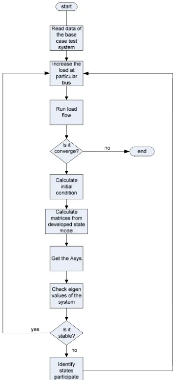
Table 3 Parameters of the generator excitation systems

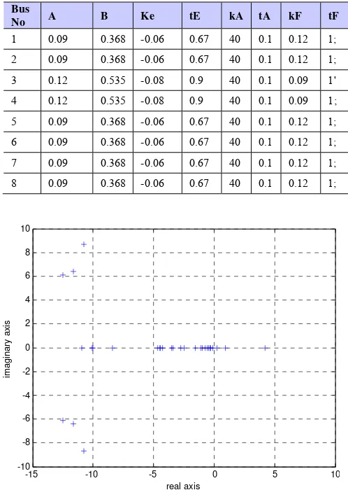
. Figure 7 Plot of eigenvalues on the base case

Table 4 Critical eigenvalues and the their participation factors on the base case

No No of

eigenvalue/mode Critical eigenvalue(s)

Participation factor

1 24 4.2152+0.0000i

δ

₁

,

δ

₈

2 37 0.9466+0.0000i

δ

₁

,

E

_q₅

3 40 0.2636+0.0000i

δ

₆

In the first time, DEPOK is loading on base case which has real load 422 KW and reactive load 174 KVAR. After running load flow, the program will calculate initial condition, then the program will generate eigenvalues of the system. The number of generator is 8, each generator has 7 states, so that we have 56 eigenvalues . Figure 7 shows the plot of eigenvalues on base case.

We plot in the range real axis from -15 to 10, and imaginary axis from -10 to 10. It is because we just concern on the positive real axis. For result of eigenvalue above, we see that there are 3 modes which has positive real part. It means those modes are unstable. For the participation factor, we have matrix 56 by 56, and we can check associated states which give big contribution to those modes. Only participation factor greater then 0.3 are listed. Those modes and their participation factor are listed in Table 4.

Table 5 Critical eigenvalues and the associated state

-15 -10 -5 0 5 10

-10 -8 -6 -4 -2 0 2 4 6 8 10

real axis

im

agi

nar

y

ax

is

Bus D H

τ

_d

′

₀

τ

q

′

0 Xq Xd

X

d

′

X

p

′

Rs _૚૙ି૜

1 2 2.64 5.69 1.5 2.02 2.11 0.28 0.49 3

2 2 3.95 9.45 1.5 2.01 2.12 0.29

7 0.5 1

3 2 2.4 9.99 0.07

1 0.573 0.88

0.27 4

0.27

3 3

4 2 3.39 8 0.06 0.69 0.93 0.30

2

0.24

5 3

5 0 2.71 4.57 0.5 1.381 1.63

9

0.25 9

0.60

4 3

6 2 3.95 9.45 1.5 2.01 2.12 2.01 0.29₇ 1

7 2 3.95 9.45 1.5 2.01 2.12 2.01 0.29

7 2

8 2 3.45 7.9 0.47 2 2.19 0.29

7

0.48

7 3

Bus

No A B Ke tE kA tA kF tF

1 0.09 0.368 -0.06 0.67 40 0.1 0.12 1;

2 0.09 0.368 -0.06 0.67 40 0.1 0.12 1;

3 0.12 0.535 -0.08 0.9 40 0.1 0.09 1'

4 0.12 0.535 -0.08 0.9 40 0.1 0.09 1;

5 0.09 0.368 -0.06 0.67 40 0.1 0.12 1;

6 0.09 0.368 -0.06 0.67 40 0.1 0.12 1;

7 0.09 0.368 -0.06 0.67 40 0.1 0.12 1;

(5)

on different loading at bus 13

Scenario Load at bus 13, DEPOK

Critical eigenvalue Associated states Mode Eigenvalues

1. 422 MW

24 4,2152+0.0000i

δ

₁

,

δ

₈

37 0,9466+0.0000i

δ

1

,

E

q5

40 0,2636+0.0000i

δ

₆

2.

844 MW (2xbase case)

24 5,08894+0.0000i

δ

₁

,

δ

₈

37 1,0403+0.0000i

E

q5

40 0,2631+0.0000i

δ

₆

3.

24 6,0130+0.0000i

δ

₁

,

δ

₈

35 1,0906+0.0000i

E

q5

40 0,2626+0.0000i

δ

₆

4.

24 6,0130+0.0000i

δ

₁

,

δ

₈

35 1,0906+0.0000i

E

_q₅

40 0,2626+0.0000i

δ

₆

5.

23 7,8396+0.0000i

δ

₁

,

δ

₈

36 1,1238+0.0000i

E

_q₅

40 0,2613+0.0000i

δ

₆

6.

2532MW (6xbase case)

23 8,6932+0.0000i

δ

₁

,

δ

₈

36 1,1218+0.0000i

E

_q₅

,

δ

₈

40 0,2605+0.0000i

δ

₆

7.

4220MW (10xbase case)

19 10,2268+6,1229i

δ

₁

,

δ

₈

20 10,2268-6,1229i

δ

₁

,

δ

₈

38 1,2268

E

_q₅

,

δ

₈

41 0,2809

δ

₆

For the base case, we see that the system is not stable due to electromechanical variable

δ

of machine 1, 6 and 8. Also the state variable

q

E

of machine 5 contributes to the instability of the system.

To see the effect of loading, we increase real load at bus 13. Start from base case (422KW), then we increase to 844 MW until 4220 MW (10 time of base case). This is the maximum loading of the scenario due to limitation of generating capacity.

From Table 5 we observe that, for increased load at bus 13, the system become more unstable. The eigenvalues are moving to positive real axis. For the last scenario, there is one complex eigenvalue. All of the unstable modes are associated with state variable

δ

of machine 1, 6 and 8, and also the state variable

E

_qof machine 5.

Due to large size of the power system, it is often necessary to construct reduced-order models for dynamic stability studies by retaining only a few modes. The appropriate definition and determination as to which state variables significantly participate in the selected modes become very important. Therefore, this study is very useful to determine state variables which give significantly participate in the selected modes.

IV.

CONCLUSION

Some notable observations regarding small-signal dynamic behaviors of the 500KV Jawa Bali power system include :

• The calculation of participation factor is very useful to identify how each dynamic variable affects a given mode or eigenvalue

• We see that after we change loading level, the dynamic performance of the system is change as the given operating conditions change, the real part of eigenvalue is bigger so that the system is more unstable.

• All of the unstable modes are associated with state variable

δ

of machine 1, 6 and 8, and also the state variable

E

_qof machine 5.

• Using participation factor we can onstruct reduced-order models for dynamic stability studies by retaining only a few modes as to which state variables significantly participate in the selected modes.

REFERENCES

[1]

K.R. Padiyar, M.A. Pai, C. Radhakrishna, “A versatile system model for the dynamic stability analysis of power systems including HVDC links”, IEEE Transaction on Power System, 1981, P: 1871-1879.

[2]

Prabha Kundur, Power System Stability and Control. New York: McGraw-Hill, Inc, 1994.

[3]

Peter W. Sauer, M.A. PAI, Power System Dynamics and Stability, Prentice Hall, 1998.

[4]

V.Vittal, M.H. Khammash, C.D. Pawloski, “Analysis of control performance for stability robustness of power system“, Proceeding of the 32nd Conference on Decision and Control, San Antonio, Texas, 1993.

[5]

Katsuhiko Ogata, Modern Control Engineering, Prentice Hall International, Inc, 1997.

[6]

P.M. Anderson, A.A Fouad, Power System Control and Stability, The Iowa State University Press, 1997

[7]

Katsuhiko Ogata, State Space Analysis of Control Systems, Prentice Hall International, Inc, 1967

[8]

William L. Brogan, Modern Control Theory, Prentice Hall International Edition, 1991.

[9]

Dr. David Banjerdpongchai, Lecture note of Control System Theory : Control System Theory, Control System Research Laboratory, 2002.

(6)

APPENDIX (The network data of 500KV Jawa Bali Power System)

1. Bus Data Bus Name Bus

No Type Pd Qd Gs Bs Area Vm Va baseKV Zone Vmax Vmin

SLAYA7 1 3 120 18 0 0 1 1 0 500 1 1.05 0.95

MTWAR7 2 2 0 0 0 0 1 1 0 500 1 1.05 0.95

CRATA7 3 2 478 246 0 0 1 1 0 500 1 1.05 0.95

SGLNG7 4 2 0 0 0 0 1 1 0 500 1 1.05 0.95

TJATI7 5 2 0 0 0 0 1 1 0 500 1 1.05 0.95

GRATI7 6 2 278 -87 0 0 1 1 0 500 1 1.05 0.95

GRSIK7 7 2 96 -65 0 0 1 1 0 500 1 1.05 0.95

PITON7 8 2 566 70 0 0 1 1 0 500 1 1.05 0.95

BKASI7 9 1 468 272 0 0 1 1 0 500 1 1.05 0.95

CIBNG7 10 1 560 470 0 0 1 1 0 500 1 1.05 0.95

CLGON7 11 1 126 22 0 0 1 1 0 500 1 1.05 0.95

CWANG7 12 1 642 312 0 0 1 1 0 500 1 1.05 0.95

DEPOK7 13 1 422 174 0 0 1 1 0 500 1 1.05 0.95

GNDUL7 14 1 765 -171 0 0 1 1 0 500 1 1.05 0.95

KMBNG7 15 1 358 168 0 0 1 1 0 500 1 1.05 0.95

BDSLN7 16 1 556 28 0 0 1 1 0 500 1 1.05 0.95

CBATU7 17 1 788 324 0 0 1 1 0 500 1 1.05 0.95

MDRCN7 18 1 600 162 0 0 1 1 0 500 1 1.05 0.95

TASIK7 19 1 466 134 0 0 1 1 0 500 1 1.05 0.95

PEDAN7 20 1 654 372 0 0 1 1 0 500 1 1.05 0.95

UNGRN7 21 1 290 -36 0 0 1 1 0 500 1 1.05 0.95

KDIRI7 22 1 585 69 0 0 1 1 0 500 1 1.05 0.95

KRIAN7 23 1 876 261 0 0 1 1 0 500 1 1.05 0.95

NSLAYA 24 1 92 88 0 0 1 1 0 500 1 1.05 0.95

2. Generator Data Bus Name Bus

No

Pg Qg Qmax Qmin Vg MBase Sta Pmax Pmin

SLAYA7 1 0 0 2040 -600 1.05 100 1 3400 1230;

MTWAR7 2 1080 0 1915 -760 1.05 100 1 2941 1330;

CRATA7 3 480 0 488 -488 1.05 100 1 1008 640;

SGLNG7 4 _{300 0 440 -140 1.05}100 _{1 700} _400;

TJATI7 5 _{1320 0 720 -240 1.05}100 _{1 1320} _600;

GRATI7 6 _{405 0 326 -122 1.05}100 _{1 527} _220;

GRSIK7 7 _{900 0 660 -610 1.05}100 _{1 1050} _238;

PITON7 8 _{3210 0 1920 -840 1.05}100 _{1 3254} _1425;

3. Branch Data Branch

No

From Bus To Bus

R X B rateA rateB rateC status

1

9 10 0.00042 0.00418 0.19185 1985 1985 1985 1;

2

9 12 0.00019 0.00848 0.08498 1985 1985 1985 1;

3

14 1 0.001219 0.0121 0.56153 1985 1985 1985 1;

4

(7)

7 ₁₀ ₁₃ _0.00015 _0.00175 _{0.08092 1985 1985 1985 1;}

8 ₁₀ ₂ _0.00084 _0.00836 _{0.38444 1985 1985 1985 1;}

9 ₁₀ ₄ _0.00080 _0.00918 _{0.40852 1985 1985 1985 1;}

10 ₁₀ ₄ _0.00080 _0.00918 _{0.40852 1985 1985 1985 1;}

11 ₁₁ ₁ _0.00014 _0.00137 _{0.06472 2209 2209 2209 1;}

12 ₁₁ ₁ _0.00014 _0.00137 _{0.06472 2209 2209 2209 1;}

13 ₁₂ ₂ _0.00082 _0.00814 _{0.37438 1985 1985 1985 1;}

14 ₁₃ ₁₄ _0.00015 _0.00175 _{0.08092 1985 1985 1985 1;}

15 ₁₃ ₁₄ _0.00015 _0.00175 _{0.08092 1985 1985 1985 1;}

16 ₁₃ ₁₉ _0.00259 _0.02959 _{1.36519 2209 2209 2209 1;}

17 ₁₃ ₁₉ _0.00259 _0.02959 _{1.36519 2209 2209 2209 1;}

18 ₁₄ ₁₅ _0.00033 _0.00100 _{0.15239 2209 2209 2209 1;}

19 ₁₄ ₁₅ _0.00033 _0.00100 _{0.15239 2209 2209 2209 1;}

20 ₂ ₁₇ _0.00054 _0.00530 _{0.24362 2209 2209 2209 1;}

21 ₂ ₁₇ _0.00054 _0.00530 _{0.24362 2209 2209 2209 1;}

22 ₂₄ ₁ _0.00000 _0.00010 _{0.00000 2209 2209 2209 1;}

23 ₁₆ ₁₈ _0.00133 _0.01320 _{0.00363 1985 1985 1985 1;}

24 ₁₆ ₁₈ _0.00133 _0.01320 _{0.00363 1985 1985 1985 1;}

25 ₁₆ ₄ _0.00036 _0.00410 _{0.18928 2209 2209 2209 1;}

26 ₁₆ ₄ _0.00036 _0.00410 _{0.18928 2209 2209 2209 1;}

27 ₁₇ ₃ _0.00045 _0.00513 _{0.23643 1985 1985 1985 1;}

28 ₁₇ ₃ _0.00045 _0.00513 _{0.23643 1985 1985 1985 1;}

29 ₃ ₄ _0.00028 _0.00277 _{0.12731 1985 1985 1985 1;}

30 ₃ ₄ _0.00028 _0.00277 _{0.12731 1985 1985 1985 1;}

31 ₁₈ ₂₁ _0.00247 _0.02464 _{1.30266 1985 1985 1985 1;}

32 ₁₈ ₂₁ _0.00247 _0.02464 _{1.30266 1985 1985 1985 1;}

33 ₁₉ ₂₀ _0.00294 _0.03354 _{1.54722 2209 2209 2209 1;}

34 ₁₉ ₂₀ _0.00294 _0.03354 _{1.54722 2209 2209 2209 1;}

35 ₂₀ ₂₁ _0.00090 _0.00840 _{0.37944 1985 1985 1985 1;}

36 ₂₀ ₂₂ _0.00200 _0.01900 _{1.02646 2209 2209 2209 1;}

37 ₂₀ ₂₂ _0.00200 _0.01900 _{1.02646 2209 2209 2209 1;}

38 ₅ ₂₁ _0.00134 _0.01534 _{0.70786 2209 2209 2209 1;}

39 ₅ ₂₁ _0.00134 _0.01534 _{0.70786 2209 2209 2209 1;}

40 ₂₁ ₂₃ _0.00290 _0.02830 _{1.26977 1985 1985 1985 1;}

41 ₆ ₂₃ _0.00089 _0.00880 _{0.40152 2209 2209 2209 1;}

42 ₆ ₂₃ _0.00089 _0.00880 _{0.40152 2209 2209 2209 1;}

43 ₆ ₈ _0.00089 _0.00880 _{0.44917 2209 2209 2209 1;}

44 ₆ ₈ _0.00089 _0.00880 _{0.44917 2209 2209 2209 1;}

45 ₇ ₂₃ _0.00030 _0.00250 _{0.12094 1985 1985 1985 1;}

46 ₇ ₂₃ _0.00030 _0.00250 _{0.12094 1985 1985 1985 1;}

47 ₂₂ ₈ _0.00120 _0.01110 _{1.01126 2209 2209 2209 1;}