SMOOTHING PARAMETER ESTIMATION FOR MARKOV RANDOM FIELD
CLASSIFICATION OF NON-GAUSSIAN DISTRIBUTION IMAGE
H. Aghighia,c∗, J. Trindera, K. Wanga, Y. Tarabalkab, S. Lima
aSchool of Civil and Environmental Engineering, The University of New South Wales, UNSW SYDNEY NSW 2052, Australia [email protected], [email protected], [email protected], [email protected]
b Inria Sophia-Antipolis M´editerran´ee, AYIN team, 06902 Sophia Antipolis, France- [email protected] cDepartment of Remote Sensing & GIS, Faculty of Earth science, Shahid Beheshti University, Tehran, Iran
Commission VII, WG VII/4
KEY WORDS:Markov random field, smoothing parameter,SVM, non-Gaussian distribution
ABSTRACT:
In the context of remote sensing image classification, Markov random fields (MRFs) have been used to combine both spectral and contextual information. TheMRFsuse a smoothing parameter to balance the contribution of the spectral versus spatial energies, which is often defined empirically. This paper proposes a framework to estimate the smoothing parameter using the probability estimates from support vector machines and the spatial class co-occurrence distribution. Furthermore, we construct a spatially weighted parameter to preserve the edges by using seven different edge detectors. The performance of the proposed methods is evaluated on two hyperspectral datasets recorded by the AVIRIS and ROSIS and a simulated ALOS PALSAR image. The experimental results demonstrated that the estimated smoothing parameter is optimal and produces a classified map with high accuracy. Moreover, we found that the Canny-based edge probability map preserved the contours better than others.
1. INTRODUCTION
Hyperspectral imaging sensors provide a huge amount of data with rich spatial, spectral and temporal resolution information. These images have attracted much attention in the remote sens-ing community and have opened the doors to variety of new ap-plications and challenges, which need to employ both spectral and spatial information for accurate data analysis and classifica-tion (Camps-Valls et al., 2014). Markov random fields (MRFs) as undirected graphical models are common methods for incor-porating both spectral and contextual information (Chen et al., 2010a). They are formulated as the minimization of an energy function which consists of spectral and spatial energy terms and an important term which plays a key controlling role known as smoothing parameter (Aghighi et al., 2014). Larger values of the smoothing parameter result in over-smoothed classified maps and too small values do not fully utilize the available spatial informa-tion (Tolpekin and Stein, 2009). Several attempts have been made to estimate the smoothing parameter, which would maximize the image classification accuracy. Derin and Elliott (1987) employed the least squares method, but the performance of their method was limited by the choice of suitable data samples (Derin and El-liott, 1987, Tso and Mather, 1999). A number of studies have ex-amined heuristic optimization algorithms to estimate the smooth-ing parameters, such as iterative conditional estimation (Salzen-stein and Pieczynski, 1997), genetic algorithms (Tso and Mather, 1999), simulated annealing (Li et al., 2012), and Ho-Kashyap optimization method which was used for automatic weight pa-rameters determination in the context of supervised classification by using training data (Serpico and Moser, 2006). In the recent years, Tolpekin and Stein (2009) demonstrated a new smooth-ing parameter estimation technique for super-resolution mappsmooth-ing based on class separability, the neighbourhood system size and the configuration of class labels. Then, Li et al. (2012) added lo-cal properties in estimating the optimal smoothing parameter and developed their spatial adaptive method. However, both
meth-∗Corresponding author.
ods introduced another parameter, which was set as a constant empirical value. Moreover, both methods suffered from simi-lar covariance assumptions for the classes. Thus, we proposed a robust smoothing parameter estimation framework to overcome their limitations (Aghighi et al., 2014). One of the limitations of the described methods is that they were developed based on the assumption of the Gaussian class conditional distribution (Aghighi et al., 2014), (Tolpekin and Stein, 2009) and (Li et al., 2012). Al-though the Gaussian distribution is widely applied in many of image labelling applications, this assumption may not be tenable for remotely sensed mixed pixels (Xu et al., 2005). Moreover, some practical data such as polarimetric synthetic aperture radar (PolSAR) data are non-Gaussian (Doulgeris et al., 2008). Another common drawback of contextual based classification ap-proaches is that they generate unreliable classification results near edges between the land covers (Moser et al., 2013), or remove the edges of small features. Therefore, several attempts have been made to develop the edge-preserving methods, which have been used during theMRFoptimization process. For instance, line processes (Moser et al., 2013) and (Solberg et al., 1996) and adaptive neighborhood systems (Hegarat-Mascle et al., 2007), are both based on the assumption of using an ideal edge map. How-ever, each image band may provide different or even conflict-ing information based on its wavelength. Therefore, some other methods such asfuzzy no-edge/edgefunction using Sobel mask (Tarabalka et al., 2010), edge probability map using Canny oper-ator (Aghighi et al., 2014) and graduated increase edge penalty (Yu and Clausi, 2008) were introduced in previous studies.
(CLCMC) and global class label co-occurrence matrix of the cat-egories (GCLCMC), which can all be computed using pairwise coupling of probability estimates from support vector machines (SVM) one-versus-one classification outputs. Furthermore, we compared seven different edge filters to incorporate the edge in-formation into theMRFframework: Canny, Sobel, Roberts, Pre-witt, Laplacian of Gaussian, curvature edge indicator, graduated edge penalty. The performance of the proposed method is eval-uated using two hyperspectral images collected by the Airborne Visible/Infrared Imaging Spectrometer (AVIRIS) and the Reflec-tive Optics System Imaging Spectrometer (ROSIS) (Section 3). Finally, conclusions are drawn in Section 4.
2. PROPOSED METHOD
In the development of our new smoothing parameter estimation framework, we denote an image byY=
Yi∈RB,i=1,2,···,m , whereB is a number of spectral channels, andmis a number of pixels. LetΩ={ω1,ω2, . . . ,ωM} be a set of M thematic classes of interest. The classification task consists in assigning for each pixelYia class labellj, yielding the classification map
L={ℓj,j=1,2,···,m}.
2.1 The Potts MRF model
The optimal classification mapL∗given the imageY can be gen-erated by solving the maximization problem for the a posteriori probability (MAP) decision rule (1).
L∗=argmax
L {
p(L|Y)}=argmax
L {
p(Y|L)p(L)} (1)
where, p(Y |L)is the class-conditional distribution and p(L)is the prior probability distribution. Based on the complexity of (1) which involves the optimization of a global distribution model of the image and due to the equivalence ofMRFand Gibbs ran-dom field (Duggin and Robinove, 1990), (Geman and Geman, 1984), this optimization problem can be simplified and resolved by minimizing the sum of local posterior energies (2) (Geman and Geman, 1984):
U(L|Y) =U(Y|L) +U(L). (2)
In this research, we applied expectation-maximization (EM) al-gorithm (Levitan and Herman, 1987) to compute theMAP. In Equation (2),U(Y|L)andU(L)denote spectral and spatial en-ergy terms, respectively. The spatial termU(L) is defined by using the Potts model, which penalizes different class labels for neighboring pixels (3):
U(L) =
∑
Yj∈Ni
W ℓj 1−δ ℓi, ℓj (3)
where,ℓjis the class label of a pixelYjwhich is a member of the symmetric neighborhood for pixelYidenoted byNi. In this equation,δ ℓi, ℓjis the Kronecker delta function (δ ℓi, ℓj= 1 i f ℓi=ℓj and δ ℓi, ℓj=0 i f ℓi6=ℓj. In Equation (3), W(ℓj)denotes the weight of contribution from pixelℓj∈Nito the spatial energy term and can be modeled as:
W ℓj
=1. In these equations,q
con-trols the overall magnitude of weights and consequently the spa-tial energies; thus, larger values ofqleads to smoother solutions (Tolpekin and Stein, 2009). Here,φ ℓj
inversely depends to d ℓi, ℓj
which is a geometric distance between the pixelℓiand
its spatial neighborsℓj( 5) (Li et al., 2012).
where,ris the spatial resolution,ηis a normalization constant to ∑
We callq/(1+q)smoothing parameter and denote it byλ; there-fore, 1/(1+q)can be written as 1−λ. As mentioned, the opti-mal classified mapL∗depends on the maximization of the poste-rior probability (1) or the minimization of local posteposte-rior energies (2 or 7), thus the absolute value ofU(L|Y)in (7) is not
impor-The spectral energyU(Y|L)can be computed as (9) (Tarabalka et al., 2010):
U(Y|L) =−ln{P(Yi|ℓi)} (9)
In order to estimate the smoothing parameter, consider that a given pixeliwith the true labelℓi=α is assigned to an incor-rect class labelℓi=β. Therefore, based on (1) we can infer that:
p(ℓi=β|Yi)≤p(ℓi=α|Yi) (10)
Which is same as (11)
U(ℓi=α|Yi)≥U(ℓi=β|Yi) (11)
By substituting the corresponding terms in (11) and solving this inequality equation, we will have the local likelihood energy change ∆Uαβι and the change of a local prior energy which is simplified
as∆UαβP =qψαβ. Furthermore,λfor each pair of classes (αand
β) can be estimated by (12) (Aghighi et al., 2014):
λαβ=
1 1+∆ψαβUl
αβ
(12)
Due to the assumption of Gaussian class conditional densities, the value of∆Uαβι was defined as a Mahalanobis distance us-ing the equal covariance matrix for all the classes in the case of (Tolpekin and Stein, 2009, Li et al., 2012); or using the mean of the covariance of each pair of classes in the case of (Aghighi et al., 2014). However, this assumption may not be tenable for remotely sensed mixed pixels (Xu et al., 2005). Thus, in order to avoid the Gaussian distribution assumption we propose a new equation to compute the change in the likelihood energy as:
∆Uαβι =−ln|{P(Yi|ℓi=β)} − {P(Yi|ℓi=α)}| (13)
catego-Table 1: Global matrix of∆Uαβι for the image’s selected pixels
∆U1ι,1=0 ∆U1ι,2 . . . ∆U1ι,M
∆U2ι,1 ∆U2ι,2=0 . . . ∆U2ι,M
. . . 0 . . .
∆UM,ι 1 ∆UM,ι 2 . . . ∆UM,Mι =0
rized based on the computed class labels and the pixels of each category are sorted in descending order based on the maximum probability in each pixel. Then, by employing theSVM accu-racy assessment results, the minimum value between user and producer accuracies of each class are used to select the propor-tion of pixels with the higher probability in each category. These selected pixels in each category are assumed to be reliably clas-sified.
For a given pixel amongst the selected pixels of each category, the maximum probability should belong to theP(Yi|ℓi=α)and other probabilities of that pixel belong toP(Yi|ℓi=β). Then the means of pixels in each category were computed using∆Uαβι (13). In the next step, each mean vector of∆Uαβι is normalized and a square matrix of∆Uαβι with sizeM was generated (see Table 1). This matrix is a zero diagonal square matrix, because each element on its diagonal indicates∆Uααι is zero.
Then, the class label of the neighbours of each pixel in each cate-gory are extracted to compute theCLCMCandGCLCMC, which are square matrices of sizeM. LetNPbe the number of pixels for a classωi; since the second orderMRFneighboring system is chosen, each pixelYiis surrounded byNS=8 pixelsYi. The
CLCMCindex is calculated for pixels of each classωias:
CLCMCCωi,ωj=
CLCMCωi,ωj shows the probability of co-occurrence of classωi
with other classesωj. In this equation,ℓcis the class label of a given pixel (i) of the category andℓsis the class label of surround-ing pixels. Due to theMRFneighboring concept which says that 1) a site cannot be a neighbor with itselfi∈/Ni′; and 2) the neigh-borhood relationship is mutual(i∈Nj⇐⇒j∈Ni)(Levitan and Herman, 1987),CLCMCis converted toGCLCMCto show the global spatial frequency distribution of each pair of classes in the image:
GCLCMCωi,ωj=CLCMCωi,ωj+CLCMCωj,ωi (15)
The index ofGCLCMCindicates the probability that a given pixel with true label (α) is misclassified as a false label (β) due to the spatial energy. Therefore,ψαβ for each pair of classes (ψαβ) is
the corresponding element ofGCLCMCmatrix for classesαand β. Although the general concepts of theCLCMCandGCLCMC indexes are similar to the concepts of class label co-occurrence matrix of the blocks (CLCMB) and global class label co-occurrence matrix of the blocks (GCLCMB) which we proposed earlier (Aghighi et al., 2014), for this paper bothCLCMCandGCLCMCare nor-malized and indicate the probability of co-occurrence of classωi with another classesωjin each category over the whole image.
In the next step, the global matrix∆Uαβι and ψαβ are used to computeλαβ for each pair of classes using Eq. (12). Finally, the
optimized smoothing parameterλ∗is computed by averaging the estimated smoothing parameterλαβfor each pair of classes ( 16)
(Aghighi et al., 2014):
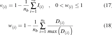
The first step for preserving the edges is to determine the edge lo-cations. Hence, we employed five of the best known edge detec-tion methods including to Canny (Canny, 1986), Sobel (Roushdy, 2006), Roberts (Jain et al., 1995), Prewitt (Prewitt, 1970), Lapla-cian of Gaussian (Marr and Hildreth, 1980) to extract the binary edge mapIi, as well as utilize the different curvature indicators to generate the curvature edge indicatorDiin each case (21) (Chen et al., 2010b). Since conflicting information is derived from the different wavelengths in hyperspectral images, Ii and Di were computed for each image band (B-band). Then a one-band edge probability map from theB-band image (nb) is computed by us-ing (17) for the Canny, Sobel, Roberts, Prewitt and Laplacian of Gaussian as well as (18) for different curvature indicators.
w(i)=1−
In order to preserve the small structures and edges in the classified map, the spatial energy component (3) can be formulated as (19 or 20)(Aghighi et al., 2014).
UspatialE (Yi) =
∑
where the superscriptErefers to the edge probability map and w(i)can be computed using (17 or 18) based on edge detection method andg(∇s)can be calculated using (24).
2.3 Different curvature indicator
This edge indicator was developed by Chen et al (2010) and called different curvature indicator. It can effectively distinguish edges from areas with flat and ramp intensity distributions in the image data (Chen et al., 2010b). The difference curvatureDifor a given pixeliof the image is defined as:
D(i)=
whereuηηanduεε represent the second derivation of the
gradi-ent∇uand perpendicular to∇u, respectively, and|.|denotes the absolute value
In these equations,uxanduxxdenote the first and second deriva-tion inx, respectively,uyanduyyare the first and second deriva-tion iny, respectively, anduxyindicates the first derivation iny of the first derivation inx. Table 2 summarizes the behaviour analysis of the different curvature edge indicator.
2.4 Graduated edge penalty
Table 2: Behaviour analysis of the different curvature edge indi-cator (Chen et al., 2010)
uηη uεε Di Edge pixel large small large Flat and ramp pixel small small small Noise pixel large large small
as the edge strength increases between two groups of pixels as-signed to different classes; thus all the edges pixels are not pe-nalized equally. The penalty function is formulated as (Yu and Clausi, 2008):
g(∇s) =e−(∇s/K)
2
, (24)
where∇s represents the normalized gradient magnitude (∇s∈
[0,1]) as the edge strength measurement on sites.Kis a positive value that controls the strength of the edge penalty term. By in-creasingKto infinity, all the edges penalties are equal to 1; and by gradually increasingK, the edges are penalized differently based on the strength or weakness of the edge gradient magnitude (Yu and Clausi, 2008). In order to calculate∇s, Equation (25) which is based on the gradient magnitude√ϑ on site s was used (Yu et al., 2012):
whereϑ can be computed using (Lee and Cok, 1991):
ϑ=1
Each of the variables of (26) can be estimated as:
ps=
In order to computeϑ, its items can be calculated using:
psqs−ts2=
∂y denote the first partial derivatives of the
bthunivariate band of imageY on siteiwith respect to vertical and horizontal directions.
3. EXPERIMENTAL RESULTS AND DISCUSSION
In order to compare the performance of the proposed method with our previous method (Aghighi et al., 2014), the same sets of train-ing and test pixels for each image were selected by the stratified random method (Foody, 2004), which can be found in (Aghighi et al., 2014). In this research, two benchmark hyperspectral datasets and all classes were collected to evaluate the proposed smoothing parameter estimation method.
1) The Indian Pines image: This hyperspectral image was recorded by the AVIRIS sensor from Indian Pines test site which was an agricultural area in North-western Indiana, USA. The image com-prises 145 by 145 pixels with 20 m/pixel spatial resolution and 200 spectral bands within a wavelength range of 0.4 to 2.5 m. The reference map contains sixteen classes, namely Alfalfa, Corn-notill, Corn-min, Corn, Grass-pasture, Grass-trees, Grass-pasture-mowed, Hay-windrowed, Oats, Soybean-notill, Soybean-mintill, Soybean clean, Wheat, Woods, Buildings-Grass-Trees-Drives and Stone-Steel-Towers.
2) The Pavia University image: The Pavia University hyperspec-tral image was recorded by ROSIS sensor from Pavia district in north Italy (Figure 2(a)). This dataset comprising of 610 by 340 pixels with spatial resolution of 1.3m and 103 spectral bands. The reference map (Figure 2(b)) contains sixteen classes, namely as-phalt, meadows, gravel, trees, painted metal sheets, bare soil, bi-tumen, self-blocking bricks and shadows.
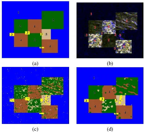
In order to evaluate the procedure on non-Gaussian data, we also simulated a 210 by 250 pixel test image using fully polarized L-band data from Phased Array typeL-band Synthetic Aperture Radar (PALSAR) sensor at the Japanese Advanced Land Observ-ing Satellite (ALOS)(Pantze et al., 2014). The quad polarizations data (HH, HV, VH and VV) was selected to reach the best clas-sification results (Doulgeris et al., 2011). After pre-processing of the data using software package (NEST version 5.0.12) provided by ESA (European Space Agency), some samples of five class, namely water, forest, urban, farm and open field were extracted. Then, they utilized to produce a simulated PALSAR data (Fig. 1(b)), such that each class has at least on boundary to every other classes (Fig. 1(a)) (Doulgeris et al., 2011). The produced data is non-Gaussian distributed due to using high resolution image and highly textured regions (Doulgeris et al., 2011).
(a) (b)
(c) (d)
Figure 1: Simulated PALSAR data . (a) Reference data ((1) wa-ter, (2) Forest, (3) Farm, (4) Urban and (5) Open field). (b) Sim-ulated image (R (VH), G (HV), and B (HH)). (c)SVMpixelwise classification map. (d)SVMMRFclassification map.
ALOS PALSAR data (Sambodo and Indriasari, 2014). The opti-malSVMparameterCandγwere chosen by fivefold cross valida-tion (Aghighi et al., 2014). TheSVMLIBlibrary (Chang and Lin, 2011) was used to estimate the probability of individual classes for each pixel and produce the classification map (see Fig. 1(c) and Fig. 1(c)). Then, the results ofSVM classification were used to estimate the smoothing parameterλ∗for both hyperspec-tral dataset and classify the image using MRF (Table 3). The smoothing parameters for simulated PALASAR data were esti-mated based on the current method and (Aghighi et al., 2014) (Table 4).
Table 3: The estimated smoothing parameter (λ∗) forMRF Studying area Indian pines Pavia University
λ∗ 0.976 0.943
Table 4: The estimated smoothing parameter (λ∗) for simulated ALOS PALASAR data
Methodology (Aghighi et al., 2014) Current method
λ∗ 0.785 0.895
In order to compare the efficiency of the proposed parameter es-timation method with (Aghighi et al., 2014) and (Tarabalka et al., 2010), both hyperspectral datasets were used. Then, theλ∗value derived in this paper was employed to manage the contribution of spectral and spatial energies for the both non-edge basedMRF method (Fig. 1(d)) and the edge-based MRF (Fig. 1(e)) by us-ing our previous edge probability map (Aghighi et al., 2014) (see Table 5).
The difference between results obtained by applying the proposed method and (Aghighi et al., 2014) are about -0.48 precent and with (Tarabalka et al., 2010) are+2.8 precents. Furthermore, comparisons of the accuracy of maps produced usingλ∗ and those produced by (Tarabalka et al., 2010) show that the overall accuracy of the classification bySVMMRF Efor the University of Pavia data have increased by 6.27 percent and 0.1 percent for the Indian Pines data (Table 5). Then we evaluated the statistical significance for each pair of corresponding classification maps in terms of accuracy by usingMcNemarstest with the 5% signifi-cance level (Zhang et al., 2011). Due to the calculatedχ2andZ values, the null hypothesis (H0) of no significant difference be-tween two corresponding maps accuracy values of this paper and (Aghighi et al., 2014) is not rejected for both Indian Pines and University of Pavia images. However, the null hypothesis (H0) of no significant difference between two corresponding maps ac-curacy values of this paper and (Tarabalka et al., 2010) for the University of Pavia is rejected.
In another experiment for non-Gaussian dataset, we utilizedSVMMRF to classify PALSAR simulated image using both estimated smooth-ing parameters (Table 4). The difference between results derived byλ∗and (Aghighi et al., 2014) is about 1.9 percent (Table 6).
We evaluated the statistical significance for both Pines and Uni-versity of Pavia classified maps in terms of accuracy by using Mc-Nemarstest with the 5% significance level (Zhang et al., 2011). According to the calculatedχ2andZvalues, the null hypothesis (H0) of no significant difference between the classified map ac-curacy values usingλ∗and (Aghighi et al., 2014) is not rejected. Moreover, the classification accuracy in percentage for each class of for PALSAR images is presented in Table 7).
As mentioned in Section 2.2, different edge preserving maps are produced using Canny, Sobel, Roberts, Prewitt, Laplacian of Gaus-sian operators, different curvature indicator and the graduated
Table 5: Overall accuracy assessment of the classified maps for SVMMRF method with different smoothing parameters and SVM for AVIRIS and ROSIS images
Smoothing Indian pines Pavia University
Parameter SV MMRF SV MMRF
NE E NE E
(Aghighi et al., 2014) 91.8 92.3 91.5 94.1 (Tarabalka et al., 2010) 92.1 91.8 86.9 87.6
λ∗ 91.2 91.9 90.8 93.9
SVM 82.2 82.2 82.2 82.2
edge penalty (17, 18, 24). Then, the new edge preserving in-formation was incorporated in theMRFusing the spatial energy term (19, 20) to produce theSVMMRF Emaps (Table 8).
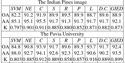
Table 8 reports the global classification accuracies for all the datasets using seven edge preserving methods. The computed overall accuracies andKappacoefficients in this research show thatSVMMRF Eusing the edge probability map, in particular the Canny edge method (Aghighi et al., 2014) results in the best overall classification accuracies in these experiments. Then, Mc-Nemarstest with the 5% significance level (Zhang et al., 2011) is used to evaluate the statistical significance betweenSVMMRF Eusing Canny based edge probability map and other edge pre-serving method. Due to the calculatedχ2andZvalues, the null hypothesis (H0) of no significant difference between Canny based edge preserving method and others is not rejected for the Univer-sity of Pavia image. However, the performance of the edge pre-serving method depends on the datasets, the land cover classes and the size of misclassified regions in the initial pixelwise clas-sification map.
Table 6: Overall accuracy assessment of the classified maps for PALSAR images
SmoothingParameter PALSAR Simulated Image Accuracy (%) (Aghighi et al., 2014) 94.2
λ∗ 96.1
SVM 91.4
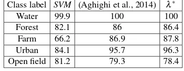
Table 7: Overall accuracy assessment of the classified maps for PALSAR images
Class label SVM (Aghighi et al., 2014) λ∗
Water 99.9 100 100
Forest 82.1 86 86.4
Farm 66.2 86.9 87.8
Urban 84.1 95.7 96.3
Open field 81.2 79.3 78.4
4. CONCLUSION
(a) (b) (c) (d) (e)
Figure 2: The University of Pavia. (a) Three-band colour composite. (b) Reference data. (c)SVMpixelwise classification map. (d) SVMMRF-NEclassification map . (e)SVMMRF-Eclassification map.
Table 8: Overall accuracy assessment of the classified maps for SVMMRF NEandSVMMRF Emethod using different edge pre-serving methods;OA(Overall accuracy),AA(Average accuracy), NE(SVMMRF NE),C(Canny),S(Sobel),R(Roberts),P (Pre-witt),L(Laplacian of Gaussian),D.C.(Different curvature indi-cator) andGIED(Graduated edge penalty)
The Indian Pines image
SVM NE C S R P L D.C. GIED OA 82.2 91.2 91.9 89.9 89.5 89.9 88.7 89.6 88.9 AA 85.1 95.1 95.5 91.7 91.3 91.7 91.7 91.7 92.1 K 0.797 0.901 0.911 0.885 0.880 0.852 0.871 0.882 0.873
The Pavia University
SVM NE C S R P L D.C. GIED OA 84.8 90.8 93.9 91.7 89.6 89.5 93.7 91.7 92.4 AA 88.0 92.7 94.1 92.6 92.3 92.3 90.6 90.2 93.5 K 0.803 0.885 0.912 0.889 0.858 0.857 0.916 0.889 0.899
smoothing parameter for both non-Gaussian and Gaussian dis-tributed data. Furthermore, the edge probability map using Canny filter yields accurate classification maps for both hyperspectral datasets.
ACKNOWLEDGMENTS
The authors would like to thank anonymous reviewers for com-ments which helped to improve and clarify this manuscript.
REFERENCES
Aghighi, H., Trinder, J., Tarabalka, Y. and Lim, S., 2014. Dy-namic block-based parameter estimation for mrf classification of high-resolution images. Geoscience and Remote Sensing Letters, IEEE 11(10), pp. 1687–1691.
Camps-Valls, G., Tuia, D., Bruzzone, L. and Benediktsson, J., 2014. Advances in hyperspectral image classification: Earth monitoring with statistical learning methods. Signal Processing Magazine, IEEE 31(1), pp. 45–54.
Canny, J., 1986. A computational approach to edge detection. Pattern Analysis and Machine Intelligence, IEEE Transactions on (6), pp. 679–698.
Chang, C.-C. and Lin, C.-J., 2011. Libsvm: a library for support vector machines. ACM Transactions on Intelligent Systems and Technology (TIST) 2(3), pp. 27.
Chen, Q., Montesinos, P., Sun, Q. S., Heng, P. A. and Xia, D. S., 2010a. Adaptive total variation denoising based on difference curvature. Image and vision computing 28(3), pp. 298–306.
Chen, Q., Montesinos, P., Sun, Q. S., Heng, P. A. and Xia, D. S., 2010b. Adaptive total variation denoising based on difference curvature. Image and vision computing 28(3), pp. 298–306.
Derin, H. and Elliott, H., 1987. Modeling and segmentation of noisy and textured images using gibbs random fields. Pattern Analysis and Machine Intelligence, IEEE Transactions on PAMI-9(1), pp. 39–55.
Doulgeris, A. P., Anfinsen, S. N. and Eltoft, T., 2008. Classifica-tion with a non-gaussian model for polsar data. Geoscience and Remote Sensing, IEEE Transactions on 46(10), pp. 2999–3009.
Doulgeris, A. P., Anfinsen, S. N. and Eltoft, T., 2011. Automated non-gaussian clustering of polarimetric synthetic aperture radar images. Geoscience and Remote Sensing, IEEE Transactions on 49(10), pp. 3665–3676.
Duggin, M. J. and Robinove, C. J., 1990. Assumptions implicit in remote sensing data acquisition and analysis. International Jour-nal of Remote Sensing 11(10), pp. 1669–1694.
Foody, G. M., 2004. Thematic map comparison: Evaluating the statistical significance of differences in classification accu-racy. Photogrammetric Engineering and remote sensing 70(5), pp. 627–633.
Geman, S. and Geman, D., 1984. Stochastic relaxation, gibbs dis-tributions, and the bayesian restoration of images. Pattern Analy-sis and Machine Intelligence, IEEE Transactions on (6), pp. 721– 741.
Hegarat-Mascle, L., Kallel, A. and Descombes, X., 2007. Ant colony optimization for image regularization based on a nonsta-tionary markov modeling. Image Processing, IEEE Transactions on 16(3), pp. 865–878.
Jain, R., Kasturi, R. and Schunck, B. G., 1995. Machine vision, vol. 5.
Lee, H.-C. and Cok, D. R., 1991. Detecting boundaries in a vector field. Signal Processing, IEEE Transactions on 39(5), pp. 1181– 1194.
Li, X., Du, Y. and Ling, F., 2012. Spatially adaptive smooth-ing parameter selection for markov random field based sub-pixel mapping of remotely sensed images. International Journal of Re-mote Sensing 33(24), pp. 7886–7901.
Marr, D. and Hildreth, E., 1980. Theory of edge detection. Pro-ceedings of the Royal Society of London. Series B. Biological Sciences 207(1167), pp. 187–217.
Moser, G., Serpico, S. B. and Benediktsson, J. A., 2013. Land-cover mapping by markov modeling of spatialcontextual informa-tion in very-high-resoluinforma-tion remote sensing images. Proceedings of the IEEE 101(3), pp. 631–651.
Pantze, A., Santoro, M. and Fransson, J. E., 2014. Change de-tection of boreal forest using bi-temporal alos palsar backscatter data. Remote Sensing of Environment.
Prewitt, J. M., 1970. Object enhancement and extraction. Picture processing and Psychopictorics 10(1), pp. 15–19.
Roushdy, M., 2006. Comparative study of edge detection algo-rithms applying on the grayscale noisy image using morphologi-cal filter. GVIP journal 6(4), pp. 17–23.
Salzenstein, F. and Pieczynski, W., 1997. Parameter estimation in hidden fuzzy markov random fields and image segmentation. Graphical Models and Image Processing 59(4), pp. 205–220.
Sambodo, K. A. and Indriasari, N., 2014. Land cover classifica-tion of alos palsar data using support vector machine. Interna-tional Journal of Remote Sensing and Earth Sciences (IJReSES).
Serpico, S. B. and Moser, G., 2006. Weight parameter optimiza-tion by the hokashyap algorithm in mrf models for supervised im-age classification. Geoscience and Remote Sensing, IEEE Trans-actions on 44(12), pp. 3695–3705.
Solberg, A. H., Taxt, T. and Jain, A. K., 1996. A markov ran-dom field model for classification of multisource satellite im-agery. Geoscience and Remote Sensing, IEEE Transactions on 34(1), pp. 100–113.
Tarabalka, Y., Fauvel, M., Chanussot, J. and Benediktsson, J. A., 2010. Svm-and mrf-based method for accurate classification of hyperspectral images. Geoscience and Remote Sensing Letters, IEEE 7(4), pp. 736–740.
Tolpekin, V. A. and Stein, A., 2009. Quantification of the effects of land-cover-class spectral separability on the accu-racy of markov-random-field-based superresolution mapping. Geoscience and Remote Sensing, IEEE Transactions on 47(9), pp. 3283–3297.
Tso, B. C. and Mather, P. M., 1999. Classification of multisource remote sensing imagery using a genetic algorithm and markov random fields. Geoscience and Remote Sensing, IEEE Transac-tions on 37(3), pp. 1255–1260.
Wu, T.-F., Lin, C.-J. and Weng, R. C., 2004. Probability estimates for multi-class classification by pairwise coupling. Journal of Machine Learning Research 5(975-1005), pp. 4.
Xu, M., Watanachaturaporn, P., Varshney, P. K. and Arora, M. K., 2005. Decision tree regression for soft classification of remote sensing data. Remote Sensing of Environment 97(3), pp. 322– 336.
Yu, P., Qin, A. and Clausi, D. A., 2012. Unsupervised polarimet-ric sar image segmentation and classification using region grow-ing with edge penalty. Geoscience and Remote Sensgrow-ing, IEEE Transactions on 50(4), pp. 1302–1317.
Yu, Q. and Clausi, D. A., 2008. Irgs: image segmentation using edge penalties and region growing. Pattern Analysis and Machine Intelligence, IEEE Transactions on 30(12), pp. 2126–2139.