Spatial explorations of land use change
and grain production in China
Peter H. Verburg
a,∗, Youqi Chen
b, Tom (A.) Veldkamp
aaDepartment of Environmental Sciences, Wageningen University, PO Box 37, 6700 AA Wageningen, Netherlands bInstitute of Natural Resources and Regional Planning, Chinese Academy of Agricultural Sciences,
Baishiqiao Road 30, Beijing 100081, China
Abstract
Studies on land use change and food security in China have often neglected the regional variability of land use change and food production conditions. This study explores the various components of agricultural production in China in a spa-tially explicit way. Included are changes in agricultural area, multiple cropping index, input use, technical efficiency and technological change. Different research methodologies are used to analyse these components of agricultural production. The methodologies are all based on semi-empirical analyses of land use patterns in relation to biophysical and socio-economical explanatory factors. The results indicate that different processes and patterns of land use change are found in various parts of the country. Large inefficiencies in the use of agricultural inputs and relatively low input use are especially found in some of the rural, less endowed, western regions of China, which indicates that in these regions of China increases in grain yield are well possible. The spatially explicit results might help to focus agricultural policies to the appropriate regions. © 2000 Elsevier Science B.V. All rights reserved.
Keywords:China; Grain production; Land use change; Yield; Technical efficiency; Spatial modelling
1. Introduction
Land use change is central to the interest of the global environmental change research community. Land use changes influence, and are determined by, climate change, loss of biodiversity, and the sustain-ability of human–environment interactions, such as food production, water and natural resources and human health. Land use changes not only include changes in land cover, but also the manner in which the land is manipulated and the intent underlying that manipulation (Turner II et al., 1995). Manipulation of land refers to the specific way in which humans use
∗Corresponding author. Tel.:+31-317-485208;
fax:+31-317-482419.
E-mail address:[email protected] (P.H. Verburg).
vegetation, soil, and water for the purpose in question, e.g., the use of fertilisers, pesticides, and irrigation for mechanised cultivation.
Land use change in China is often seen in the light of its impact on food security. With a rising demand for agricultural products, as a consequence of popu-lation growth and changing consumption patterns, it is essential for China to increase its food production. In recent years much discussion is devoted to China’s ability to maintain food self-sufficiency (Garnaut and Ma, 1992; Brown, 1995; Rozelle and Rosegrant, 1997; Lin, 1998). China might become a major importer of food products as a consequence of its losses of agricul-tural land through urbanisation and degradation, and its limited possibilities to increase output per unit area. Brown (1995) takes the most extreme position, claim-ing that China’s grain production will fall in absolute
terms while demand will rise, creating a shortfall of more than 200 million metric tons by 2030. Other au-thors, using more sophisticated analyses, have shown that shortfalls in production are probably lower (Paarl-berg, 1997; Huang et al., 1999). Recent projections by the United States Department of Agriculture have now again sharply reduced projected growth in China’s grain import demand (USDA, 2000). The largest un-certainties in the projections of changes in China’s food economy are found on the supply side of the food balance, largely as a consequence of differences in the analysts’ perception of prospects for technological change and other factors affecting growth of cultivated land and productivity (Fan and Agcaoili-Sombilla, 1997). Almost all of these assessments of the impact of land use changes on food supply in China are based upon an analysis of the economy at the national level. Such aggregated assessments lack the analysis of re-gional variability in land use change and potentials to increase production. The highly diverse natural and socio-economic conditions in China cause land use change to have differential impacts across the country. Spatially explicit assessments are needed to identify areas that are likely to be subject to dramatic land use modifications in the near future. Such information is especially important for land use planners since, in order to focus policy interventions, one needs not only to know the present rates and localities of land use change, but also to anticipate where conversions are most likely to occur next. Such predicative informa-tion is essential to support the timely policy response. This paper studies potential near-future changes in China’s agricultural production from a spatially ex-plicit perspective. The different components of land use change influencing grain production, are studied in order to identify potential ’hot-spots’ of change. Regional variability is related to its explanatory fac-tors, to identify the processes underlying the changes in land use.
2. Methodology and data
2.1. Overview
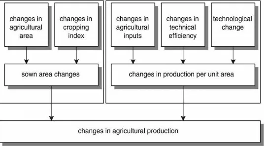
Changes in agricultural production result from changes in one or more of the components of the land use system. Changes in agricultural production
can either originate from changes in the sown area or from changes in the production level per unit of land (yield). For regions where it is possible to sow the land more than once a year, changes in sown area can be divided into changes in agricultural area and changes in the multiple cropping index. Changes in yield can be subdivided into three components. First, the traditional source of growth stems from increases in agricultural inputs, e.g., irrigation and fertilisers. The second source of growth comes from increases in the efficiency of production. Increases in production efficiency make more output available with the same amount of inputs. Institutional innovations can be an important source of efficiency growth, as these elimi-nate restraints in resource allocation. The third source of growth is technological change, which shifts the production function upward. So, similar to efficiency increases, more outputs become available out of the same amount of inputs. New, improved varieties can be an important source of technological progress. Fig. 1 shows the thus derived five sources of change in agricultural production. These different sources of change in agricultural production all have their own drivers and constraints. Therefore, the different sources of change in production have been analysed separately by different methodologies, described in more detail hereafter. Some of these methodologies have been described elaborately in other papers, so only the main characteristics are repeated here. All these methodologies have in common that they use data on the spatial variability of production conditions and (proximate) driving forces to analyse the dynam-ics of the land use system. Another similarity between the methodologies is the use of statistical methods which are used to establish relationships between the pattern of land use and its supposed driving factors. The following paragraphs describe the data sets used in the study and the different methodologies.
2.2. Data
Fig. 1. Land use change components that determine changes in grain production.
and climatic characteristics are based on maps and interpolated climate data respectively, land cover data were unfortunately only available for 1986 and 1991 whereas data on agricultural inputs and production are also available for 1996. Therefore, the base-year for all calculations is 1991, whereas 1986 and 1996 data are used to capture the temporal dynamics. The data and their various sources are summarised in Ap-pendix A of this paper and described in more detail in Verburg and Chen (2000). All data are converted into a regular grid to match the representation of the dif-ferent data and facilitate the analysis. The basic grid size, to which all data are converted, is 32×32 km (∼1000 km2), which equals the average county size in the eastern part of China. There has been consider-able discussion about the reliability of Chinese land use statistics, especially with respect to the amount of cultivated land (Crook, 1993). Official statistics have always underestimated the area of cultivated land. However, the cultivated area in the agricultural survey we have used, equals 133 million hectares, which cor-responds with the area generally assumed to be reli-able (Alexandratos, 1996; Smil, 1999). For grain yield we had to use official statistics. Underreporting of arable land in official statistics has led to inflated esti-mates of grain yields and the appearance that China’s yields are high by world standards. Statisticians have admitted that they have overstated grain yields to com-pensate for the underreported land area. They rely on sample survey cuttings to determine actual yields, and then inflate them 20–30% (Crook and Colby, 1996). The same overestimation holds for fertiliser
appli-cation rates as these are also calculated with arable areas derived from official statistics. Unfortunately, it is not possible to correct for the unreliability of the Chinese land use statistics. Any calculation presented in this paper should therefore be seen in the light of this problem. However, we believe that it is still pos-sible to use the data to indicate ‘hot-spots’ of change and make conclusions on the relative importance of the processes throughout the country.
2.3. Methodologies
2.3.1. Changes in agricultural area
Changes in agricultural area can result from the reclamation of land, e.g., forest and grassland, into agricultural land as well as from the conversion of agricultural land into other land use types through, e.g., encroachment of cities or desertification. Whereas the former conversion is constrained by availability of suitable land resources, the latter is the result of competition between land use types. To explore these changes in agricultural area for China a dynamic, spa-tially explicit land use change model is used. This model, the CLUE (Conversion of Land Use and its Effects) modelling framework, has been described in more detail in Verburg et al. (1999a) whereas the ap-plication of the model for China has been described in Verburg et al. (1999b). Therefore, in this section only the main characteristics of the modelling framework and the scenarios used in this paper are mentioned.
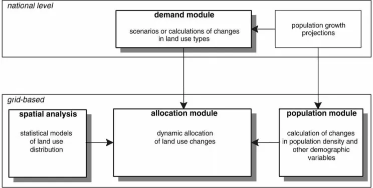
Fig. 2. General structure of the CLUE modelling framework for the spatially explicit calculation of changes in the land use change pattern.
The demand module contains, at the national level, scenarios for changes in demand for different land use types. In this study these scenarios are entirely based on previous studies published in literature. Most of these studies are based on the demand for agricul-tural products, taking into account population growth, changes in diet and import/export quantities. The pop-ulation module calculates changes in poppop-ulation and associated demographic characteristics based upon projections and historic growth rates. The central part of the model is the allocation module. This module calculates for all grid cells the changes in land use on a yearly basis. The allocation itself is based upon a spatial analysis of the complex interaction between land use, socio-economic conditions and biophysical constraints. The Appendix A gives an overview of the demographic, socio-economic, soil related, geomor-phologic and climatic variables evaluated in the anal-ysis for China. All these variables can, as is known from literature (Turner II et al., 1993), influence the distribution of land use. However, not in all situations all of these variables will add a significant contribu-tion to the explanacontribu-tion of the land use distribucontribu-tion. Therefore, a stepwise regression procedure is used to straightforwardly select variables with a significant contribution.
The allocation module uses these spatial relations to calculate changes in relative land cover, given either a
change in one of the determining factors, e.g., changes in population density or urbanisation, or a change in competitive advantage upon a change in demand at the national level. For every year the allocation module calculates changes, until the demand for the different land use types is equalled. For every grid cell alloca-tion is constrained by the total land area in the grid cell, so that competition between the land use types is explicitly taken into account.
The land use types included in the CLUE model for China are cultivated land, horticultural land, for-est, grassland, built-up land and unused land (mainly desert). In addition, a nested model run is made to simulate the relative occupation of agricultural land by different crops or groups of crops. We have mod-elled rice, wheat, corn, other grain crops, cash crops, vegetables and other crops separately.
Table 1
Baseline scenario for CLUE simulations
Demand for land cover types Area in 1991 (million hectares) Yearly change (1991–2010; 1000 ha)
Cultivated land 132 −574
Horticultural land 5 182
Forest 195 107
Grassland 256 0
Built-up land 25 221
Water 34 0
Unused 296 64
Population growth assumptions Value Source of projection
Total population 17% increase (1991–2010) US Census (1997)
%Urban population 27% (1991) to 43% (2010) UN (1995)
%Rural labour force of rural population Constant Shen and Spence (1996) %Agricultural labour force of rural labour force 78% (1991) to 65% (2010) Trend and author’s estimates
with growth rates proportional to the growth rates observed in the grid cells between 1986 and 1991.
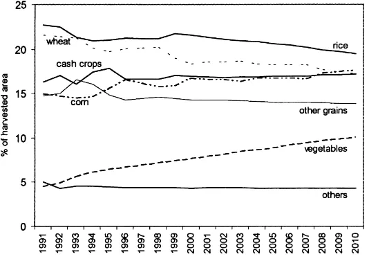
The demand for the different crop types is based on projections to 2007 by the United States Depart-ment of Agriculture (USDA, 1998) which provides yearly projections for all major crops. No projections are given for potato (included in the other grain cate-gory), some cash crops, vegetables and crops grouped in the category other crops, e.g., fodder and medici-nal crops. These crop projections are made based on trends and literature (e.g., Lin and Colby, 1996).
China is expected to become a large vegetable exporter as China has a comparative advantage in
observed data have been used, which can be seen from the fluctuations in relative harvested area.
2.3.2. Cropping index
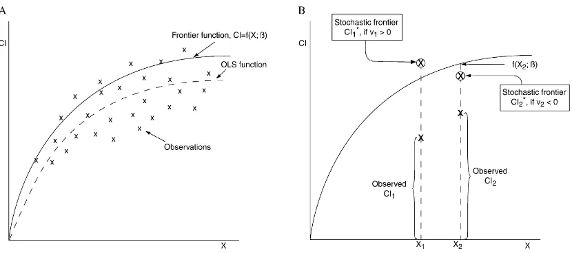
The cropping index denotes the number of times a year that a piece of land is sown to a crop. The possibil-ities for multiple cropping are constrained by climatic conditions and water availability. The temperature in winter is in a large part of China too low to support crop growth. Other parts, with more favourable tem-peratures, but with a distinct dry season, lack the water resources needed for crop growth unless irrigation is available. To understand the spatial variability in crop-ping index it is therefore essential to study both the actual and the potential cropping index. Agro-climatic and crop growth models can be used to calculate the variation in potential cropping indices throughout the country (Cao et al., 1995). However, this requires detailed information on crop growth and hydrologi-cal conditions. Because at many places China’s crop-ping systems already operate at the maximum possi-ble cropping index, it is also possipossi-ble to obtain the maximum cropping indices by an analysis of the ac-tual cropping index with a frontier function approach. Following the stochastic production function literature (Coelli et al., 1998) the following model was specified:
CIi =f (Xi, β)+vi −ui (1)
Fig. 4. Schematic representation of frontier function approach: (A) frontier function as compared to ordinary least squares (OLS) function; (B) observed multiple cropping index (CI) versus stochastic frontier value of the cropping index (adapted from Battese, 1992).
where CIiis the average cropping index in theith grid
cell, Xi denotes the vector with climatic and
hydro-logical factors determining the cropping index,vi is a
random error term which is assumed to be identically and independently distributed asN (0, σv2), andui are
non-negative truncations of theN (0, σu2)distribution (i.e., half-normal distribution). The frontier function is represented by f(Xi, β), and is a measure of the
maximum cropping index for any particular vector Xi. Both vi and ui cause the actual cropping index
to deviate from this frontier. The random variability, e.g., measurement errors or temporary constraints, is represented byvi. The non-negative error termui
rep-resents deviations from the maximum potential crop-ping index attributable to inefficiencies. Inefficiency means in these circumstances a non-optimal use of the agro-climatic conditions. The basic structure of the stochastic frontier model is depicted in Fig. 4 for a hy-pothetical relation between CI andX. Fig. 4A indicates how the frontier function might relate to an ordinary least squares function (OLS) while Fig. 4B focuses on the condition of two grid-cells, represented by 1 and 2. In grid-cell 1 a cropping index CI1is found for the agro-climatic conditions X1. The stochastic frontier cropping index, CI∗
cropping index, CI∗
2, which is less than the value of the deterministic frontier function, f(X2,β), because the random error, v2, is negative. The efficiency in an individual grid-cell is defined in terms of the ratio of the observed cropping index to the correspond-ing stochastic frontier croppcorrespond-ing index, conditional on agro-climatic conditions. Thus, the efficiency in the context of the stochastic frontier function is
TEi =
CIi
CI∗ i
(2)
where TEi is the efficiency in grid celli.
In this study the vectorXconsists of the (long-term average) yearly temperature (TMP AVG), the differ-ence in temperature between the warmest and coldest month (TMP RNG), the number of months that the av-erage monthly temperature is above 10◦C (TMP 10C),
the number of months that more than 50 mm rain is collected (PRC 50M), the average percentage of sun-shine (SUN TOT) and the fraction of all cultivated land in a certain grid cell that is irrigated (IRRI). The logarithm of the cropping index was used, because it resulted in a significantly better model fit. The frontier function is estimated for the three years that data were available with Maximum Likelihood procedures using FRONTIER4.1 software (Coelli, 1994). The actual changes in cropping index between 1986 and 1996 are used to evaluate the relevance of the calculated inefficiencies for future changes in cropping index.
2.3.3. Agricultural inputs
Farming systems can be characterised by their in-puts and outin-puts. Therefore, each grid cell is classified by the average farming intensity calculated from an analysis of agricultural inputs and outputs. A disjoint cluster analysis is used to summarise the different inputs and outputs into groups of farming systems. In the cluster analysis grain yield (YGRAIN), chem-ical fertiliser input (FERT), irrigation (IRRI), labour availability (LABOUR), mechanisation (MACH) and manure application (MANURE) are used to charac-terise the farming system groups. To understand the spatial distribution of the distinguished farming sys-tems, we have studied the spatial differences of the individual inputs and the farming system groups as a whole in relation to a number of environmental and socio-economic factors. The relation between grain yield and agricultural inputs is studied by fitting a
production function with a Cobb–Douglas functional form given by
ln(Yi)=β0+β1ln(FERTi)+β2ln(IRRIi)
+β3ln(LABOURi)+β4ln(MANUREi)
+β5ln(MACHi) (3)
2.3.4. Production efficiency
The notion of stochastic frontier functions and effi-ciency, as described in Section 2.3.2, originates from economic literature where frontier functions are used to determine the efficiency with which a firm produces a certain output given the level of inputs (Farrell, 1957; Battese, 1992; Bravo-Ureta and Pinheiro, 1993). The same holds for agricultural firms, or groups of agri-cultural firms in a certain area. Output, in this study defined as grain production per unit area (Yi), is a
function of agricultural inputs and the efficiency with which these inputs are used. Therefore, we can write
ln(Yi)=f (Xi, β)+vi −ui (4)
wheref(Xi,β) presents the frontier production
func-tion and Xi denotes the vector of agricultural inputs
similar to the Cobb–Douglas function (Section 2.3.3). vi is the random variability in production and is
iden-tically and independently distributed as N (0, σv2). The non-negative error termui represents deviations
from the frontier output attributable to technical in-efficiency. Instead of giving these deviations a fixed distribution, as we do in the function for the crop-ping index, we follow the specification of Battese and Coelli (1995) where the inefficiency effects (µi)
are expressed as an explicit function of a vector of grid-cell specific variables and a random error. There-fore,ui is assumed to be independently distributed as
truncations at zero of theN (µi, σu2)distribution. For
this study the inefficiency function is defined by
µi=δ0+δ1TMP AVGi+δ2PRC TOTi
+δ3SOILi+δ4MEANELEVi+δ5DISTCITYi
+δ6ILLITi+δ7%AGLFi+δ8INCOMEi
+δ9EROSIONi (5)
differences in climate over the country will influence crop growth and therefore the efficiency in grain pro-duction. Soil fertility (SOIL) is assumed to be impor-tant because in areas with a high natural soil fertility less fertiliser is needed to obtain the same crop yield. Furthermore, the elevation (MEANELEV) is expected to be negatively related to the efficiency as rugged terrain asks for relatively more labour and hampers cultivation practices. A second set of variables relates to the socio-economic conditions. Agriculture in areas which are relatively distant from cities (DISTCITY) is assumed to be hampered due to poor access to in-formation and appropriate inputs, causing inefficien-cies. In a similar way it is assumed that the illiteracy level (ILLIT), representative for the received educa-tion, influences efficiency. The percentage of the total population that is part of the agricultural labour force (%AGLF) is supposed to be indicative for the oppor-tunities for off-farm labour, which is thought to be related to the efficiency of grain production. Average income (INCOME) is supposed to influence efficiency by the ability the farmer has to invest in his land (e.g., terracing) and the possibilities to buy a balanced set of appropriate inputs. The extent and impact of wa-ter erosion (EROSION) is assumed to be negatively related to efficiency as erosion can damage the crops, remove nutrients and have a negative effect on soil structure.
The frontier function and efficiencies are again calculated with the use of Maximum Likelihood procedures through FRONTIER4.1 software (Coelli, 1994).
2.3.5. Technological progress
Technological progress can be defined as a shift of the production function upwards. So, out of the same amount of inputs more output becomes available. This shift can easily be defined by including a time trend variable in the following production function:
ln(Yi)=βtt+f (Xi, β) (6)
wheretis a time trend variable. The production func-tion is calculated with data for the years 1986, 1991 and 1996. Data for years in between, which would make the estimates of the coefficient for the time trend variable more robust, are not available.
3. Results and interpretations
3.1. Changes in agricultural area
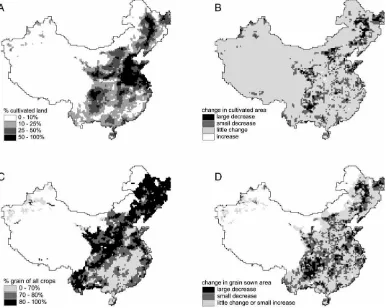
The results of the simulation of changes in the agri-cultural area with the CLUE model are presented in Fig. 5. Fig. 5A shows the spatial distribution of culti-vated land in 1991, the reference year, as derived from the agricultural survey. The distribution of changes in cultivated area as simulated for the period 1991–2010 are indicated in Fig. 5B. The results suggest that although the total extent of the cultivated area de-creases, some regions showing an increase can still be distinguished. A more extended analysis of a similar model run, as presented by Verburg et al. (1999b), indicates that in different areas different land use con-versions are responsible for the decrease in cultivated area. Degradation of arable land causes large losses of cultivated land on the Ordos Plateau of Inner Mon-golia and on the Loess Plateau. These are areas that are well known for their marginal agriculture and sus-ceptibility to degradation (Smil, 1993; Qinye et al., 1994; Liu and Lu, 1999). Other ‘hot-spots’ of land use change can be found in the main agricultural regions of east, central, south and southwest China as result of the expansion of the built-up and horticultural area. In these regions large losses of agricultural land are found around all major urban areas, especially the larger area surrounding Shanghai.
Fig. 5C displays the relative importance of grain crops in the cultivated area for 1991. Grain crops are a more important crop in the northern and western parts of China than in the central, southern and eastern parts. In the southern and eastern parts of China cash crops make up an important part of the cropping sys-tem. Decreases in the share of the area devoted to grain crops are found throughout the whole country. Promi-nent areas are, however, the urban regions of eastern and central China, where large increases in vegetable area and other cash crops are expected as a result of the growing demand for these products by the urban residents.
3.2. Cropping index
Fig. 5. (A) Cultivated land in 1991; (B) predicted changes in cultivated area between 1991 and 2010 by the CLUE model; (C) percentage of grain of harvested area in 1991; (D) changes in total grain sown area between 1991 and 2010.
Table 2
Stochastic frontier functions for cropping index in China for 1986 and 1991a
Coefficient 1986 Coefficient 1991 Coefficient 1996 Frontier function
INTERCEPT 0.168 (7.31)∗ 0.367 (15.8)∗ 0.611 (22.8)∗
TMP AVG 0.0438 (39.9)∗ 0.0416 (37.4)∗ 0.0369 (25.9)∗
TMP RNG 0.00442 (10.5)∗ 0.00253 (5.86)∗
−0.000240 (−0.462)∗
TMP 10C −0.0462 (−20.6)∗
−0.0410 (−18.0)∗
−0.0306 (−10.6)∗
PRC 50M 0.0347 (28.9)∗ 0.0342 (28.1)∗ 0.0279 (18.6)∗
SUN TOT −0.00505 (−16.7)∗
−0.00719 (−23.5)∗
−0.00941 (−24.7)∗
IRRI 0.00180 (23.6)∗ 0.00126 (15.1)∗ 0.00141 (13.8)∗
Statistical parameters
Sigma-squared (σs2=σu2+σv2) 0.0375 (26.6)
∗ 0.0349 (25.8)∗ 0.0587 (33.4)∗
Gamma (γ =σu2/σs2) 0.790 (40.7)
∗ 0.723 (30.8)∗ 0.803 (65.3)∗
Log likelihood function 2733 2683 1768
LR test of the one-sided error 171.5∗∗ 122.5∗∗ 539.0∗∗
at-Ratios between the parentheses.
∗Significant at the 0.01 level.
found at higher temperatures, longer rainy periods and a larger proportion of the cultivated area that is irri-gated. The number of months with temperatures above 10◦C and the range in temperature modify this
rela-tionship. The frontier functions for the different years are very much similar, indicating a stable relation be-tween the agro-climatic variables and the cropping in-dex. The Likelihood Ratio test statistic is calculated for testing the absence of inefficiency effects from the frontier (Coelli et al., 1998). For all three years the value is highly significant, hence the null hypothesis of no inefficiency effects is rejected. The gamma statis-tic is indicative for the partitioning of the deviations from the frontier. A zero-value forγ indicates that the deviations from the frontier are entirely due to noise, while a value of 1 would indicate that all deviations are due to inefficiency. The values found in this study (0.72–0.80) indicate that still a considerable propor-tion of the deviapropor-tions from the frontier in this study can be attributed to noise.
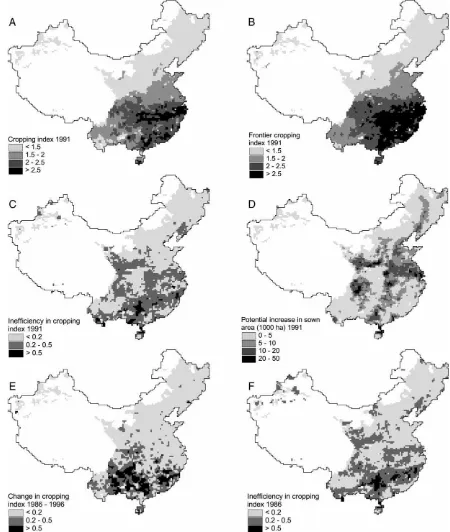
Fig. 6 presents the results in a spatially explicit way. Fig. 6A and B indicates the actual and frontier crop-ping index in 1991, respectively. The observed pattern corresponds fairly well with the climatic variability throughout the country whereas local variations are mainly due to differences in irrigation. The difference between the actual cropping index and the stochastic frontier cropping index is the inefficiency, which is in-dicated in Fig. 6C. This figure shows that most poten-tial for higher cropping indices is found in the central and southern regions of China. However, in these ar-eas the cultivated arar-eas are generally small, hence the increase in sown area upon an increase in cropping index is small. When the inefficiencies in cropping in-dex are multiplied by the cultivated area the potential increase that can be attained in sown area is indicated (Fig. 6D). As a consequence of its extended cultivated area, the North China plain area is identified as the main area where considerable increases in sown area are possible, in spite of the relatively small potential increase in cropping index. The total sown area that could be gained by increasing the cropping index to its stochastic frontier value is about 25 million hectares, which would mean an increase of about 12% in sown area.
The feasibility of increasing grain production through an increase in cropping index can be deter-mined by an analysis of the reasons underlying the
deviations from the frontier cropping index. Correla-tion analysis between the estimated efficiencies and the available socio-economic and biophysical vari-ables did not result in strong conclusions. The best relations were found with the mean elevation (−0.10, significant at 0.01 level) and the available labour per unit area of cultivated land (0.14, significant at 0.01 level), meaning that mountainous areas might ham-per high cropping intensities and that labour shortage might cause less intensive use of the land. Another reason for deviations between actual and frontier cropping index might be found in the choice of crops. Some crops, e.g., sugar cane, have a longer growing season, inhibiting multiple cropping. However for individual farmers such crops can often make much higher profits. This hypothesis is confirmed by a significant, negative correlation (−0.07) between the relative share of sugar in the cropping system and the efficiency. Because of large demands for high quality rice farmers increasingly cultivate varieties that have a much longer growing period, also decreasing the multiple cropping index. It was expected that ineffi-ciencies would also be higher near urban centres, with large possibilities for off-farm labour. However, no evidence was found in the data. It can be hypothesised that regulations by county governments that specify minimum cropping indices overrule this effect.
The potential for increases in cropping index can be seen as an indicator for near future increases of the cropping index. In Fig. 6E and F the observed changes in cropping index between 1986 and 1996 are com-pared with the potential for increase in cropping in-dex determined for 1986. If evaluated for individual grid-cells, the correlation is relatively low (0.34, sig-nificant at 0.01 level). However, the general pattern is very similar. When evaluated at the aggregated level of the seven main geographical regions of China, a correlation between the observed changes in cropping index and the potential for change of 0.83 is found. This indicates that it is probable that also for longer time periods most increases in cropping index will be found in southern China.
3.3. Agricultural inputs
Table 3
Mean value of agricultural parameters for farming system groups in China as determined by a cluster analysisa
Farming systems group
Number of cells
Grain yield (kg/ha)
Fertiliser application (kg/ha)
Irrigated (%)
Labour (persons/ hectare sown area)
Machine cultivated (%)
Manure application (ton/ha) Group 1 61 (1%) 7205 (495) 292 (74) 58 (35) 2.43 (2.47) 63 (21) 8.97 (4) Group 2 1485 (32%) 5089 (565) 218 (84) 65 (23) 3.73 (2.02) 49 (28) 9.59 (6) Group 3 2385 (51%) 3270 (611) 139 (67) 39 (25) 2.58 (1.77) 38 (30) 8.64 (5) Group 4 712 (15%) 1467 (512) 70 (80) 15 (13) 1.14 (1.00) 34 (26) 6.31 (5) Mean 4643 (100%) 3627 (1404) 156 (91) 44 (28) 2.74 (2.07) 41 (29) 8.59 (5)
aStandard deviations between the parentheses.
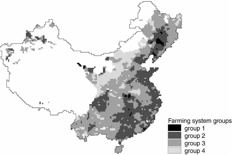
in Table 3. The groups indicate the intensity of the farming systems. Farming system groups 1 and 2 are characterised by high inputs and high yields while farming system groups 3 and 4 are characterised by low inputs and low yields. Only labour availability does not obey the general pattern. Fig. 7 shows the spatial distribution of the different farming system groups. From this map it can be seen that the farming system groups have a clear distribution throughout the country. The high input farming systems of group 1 and 2 are mainly located in the central and eastern part
Fig. 7. Farming system groups as distinguished by cluster analysis; group 1 represents the most intensive land use systems with respect to inputs and outputs whereas group 4 represents the most extensive systems (see Table 3).
Table 4
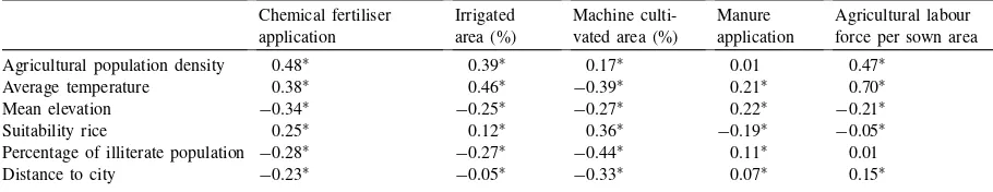
Pearson correlation coefficients between agricultural inputs and a number of biophysical and demographic factors Chemical fertiliser force per sown area Agricultural population density 0.48∗ 0.39∗ 0.17∗ 0.01 0.47∗
Average temperature 0.38∗ 0.46∗ −0.39∗ 0.21∗ 0.70∗
Mean elevation −0.34∗ −0.25∗ −0.27∗ 0.22∗ −0.21∗
Suitability rice 0.25∗ 0.12∗ 0.36∗ −0.19∗ −0.05∗
Percentage of illiterate population −0.28∗ −0.27∗ −0.44∗ 0.11∗ 0.01
Distance to city −0.23∗ −0.05∗ −0.33∗ 0.07∗ 0.15∗
∗Significant at 0.01 level.
and agricultural machinery tends to decrease with the distance to a city and increasing percentages of illiter-ate population. In areas with higher population densi-ties generally more inputs are used, probably a conse-quence of strong competition for land resources. The correlation of fertiliser and irrigation with the average temperature is a result of the location of intensively managed, irrigated rice cropping systems in the south-ern part of China. Because rice cultivation is not as mechanised as the cultivation of other grains, we find a negative correlation coefficient with temperature for mechanisation and a positive one for the labour use intensity. The connection between management intensity and soil quality is expressed by the positive correlation between soil suitability for rice cultivation and input quantities. The distribution of manure appli-cation does not obey the general pattern found. Inputs of manure are mainly determined by the availability of manure, and thus the distribution of livestock (Verburg and van Keulen, 1999). Increasing labour intensities in agriculture with the distance to city are indicative for the decreasing opportunities for off-farm labour.
Table 5 presents the Cobb–Douglas production function as was derived for grain yield in 1991. Except for LABOUR, all estimates in the production func-tion have the expected positive sign. The very small, but negative coefficient for agricultural labour force is somewhat surprising. However, low elasticities for labour are also found in other labour-rich Asian countries (Huang and Rozelle, 1995). Besides, Bhat-tacharyya and Parker (1999) and Rawski and Mead (1998) have argued that Chinese statistics massively overestimate the number of farm workers. This might well explain the negative value of the coefficient for labour in the production function. Chemical fertiliser
is the most important input factor, followed by manure and irrigation. The elasticity for agricultural mechani-sation is, however, small. These results are consistent with other studies (Yao and Liu, 1998; Fan, 1997) that also found low elasticities for machinery, probably a result of abundance of cheap agricultural labour.
From the production function it is clear that chem-ical fertiliser is the most important input in Chinese agriculture. Inputs of chemical fertiliser have rapidly risen during the recent past. However, increases in fer-tiliser use have not made an equal pace throughout the country.
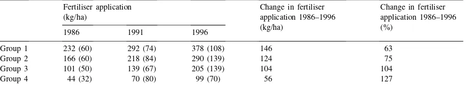
Table 6 presents the changes in fertiliser application during the period 1986–1996 for the different farming system groups. From this table it can be clearly seen that the largest (absolute) increases in fertiliser use are found in areas that already have a high fertiliser use. So, in spite of the doubling of fertiliser use in areas classified as farming system groups 3 and 4, the
Table 5
Production function for grain yield in 1991a
Variable Parameter Average function Production function
Intercept β0 5.450 (132)∗
FERT β1 0.390 (44.0)∗
IRRI β2 0.133 (18.7)∗
LABOUR β3 −0.023 (−2.91)∗
MANURE β4 0.132 (13.4)∗
MACH β5 0.012 (2.56)∗∗
F-statistic model 1430∗
Adj.R2 0.61
aValues in parentheses are thet-ratios of the estimates.
Table 6
Input use for the farming system groups in China as determined by a cluster analysisa
Fertiliser application
aStandard deviations between the parentheses.
differences in fertiliser use between the groups have increased. In the areas of farming system groups 3 and 4 both grain transportation and grain storage facilities are very backward and limited, the rural population not only has to produce food locally, but it also has to devote most of the arable land to food production for survival (Lin and Wen, 1995). So, under the present economic and infrastructural conditions in these areas, individual households are not able to increase their agricultural inputs (Lin and Li, 1995). Another reason for lower increases in fertiliser use in the areas of farming system groups 3 and 4 can be the allocation policy of subsidised fertiliser. The largest category of allocation is the ‘procurement-linked fertiliser’, its uniform price nation-wide being set by the central government. The central leadership allocates this fer-tiliser, which, as its name suggests, is directly linked to the quantity of state crop procurement. As a result, most of the subsidised urea flows into prosperous areas, where the state purchases most of its grain, cot-ton and oilseed crops. In contrast, farmers in poorer areas receive little or no subsidised urea because they have few surplus crops (Ye and Rozelle, 1994). More recently these subsidies have largely been dropped.
Given the functional form of the production func-tion and the already high levels of fertiliser use, di-minishing returns upon further increases of chemical fertiliser input in the areas of farming system groups 1 and 2 can be expected. Furthermore, excessive use of agricultural chemicals has already caused severe damages to the natural environment, e.g., groundwater pollution and deterioration of soil fertility (Jin et al., 1999; Smil, 1993). The low inputs and yields in large parts of western China suggest that there is still a vast potential for raising grain output by using more
land-augmenting inputs such as fertilisers and irriga-tion in these medium and low yield regions.
3.4. Production efficiency
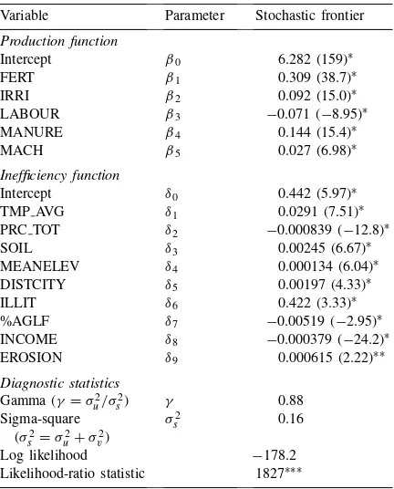
The parameters that are calculated for the fron-tier production and inefficiency function are given in Table 7. The values of the frontier production func-tion are very similar to those of the average producfunc-tion function (Table 5), indicating that the frontier func-tion consists of a near-neutral upward shift of the av-erage function. The diagnostic statistics indicate that a relatively large part of the variation is explained by inefficiency effects whereas the likelihood-ratio statis-tic is highly significant, rejecting the hypothesis of no inefficiency effect in grain production in China.
Table 7
Stochastic frontier production function for grain production in Chinaa
Variable Parameter Stochastic frontier Production function
Intercept β0 6.282 (159)∗
FERT β1 0.309 (38.7)∗
Intercept δ0 0.442 (5.97)∗
TMP AVG δ1 0.0291 (7.51)∗
PRC TOT δ2 −0.000839 (−12.8)∗
SOIL δ3 0.00245 (6.67)∗
MEANELEV δ4 0.000134 (6.04)∗
DISTCITY δ5 0.00197 (4.33)∗
ILLIT δ6 0.422 (3.33)∗
%AGLF δ7 −0.00519 (−2.95)∗
INCOME δ8 −0.000379 (−24.2)∗
EROSION δ9 0.000615 (2.22)∗∗
Diagnostic statistics
Gamma (γ =σu2/σs2) γ 0.88 Sigma-square
(σs2=σu2+σv2)
σs2 0.16
Log likelihood −178.2
Likelihood-ratio statistic 1827∗∗∗
aValues in parentheses are thet-ratios of the estimates.
∗Significant at the 0.01 level. ∗∗Significant at the 0.05 level.
∗∗∗Significant at 0.01 level according to Table 1 of Kodde and
Palm (1986).
on production efficiency. This suggests that the pos-sibilities for non-farm labour decrease the technical efficiency of grain production. Income is an important variable in the inefficiency function, having a positive effect on the efficiency of input use, probably through the opportunities to buy higher quality, more balanced inputs and invest in the land (e.g., terracing). In cor-respondence with other studies (Yao and Liu, 1998; Lambert and Parker, 1998), we found that erosion is also an important source of inefficiency in agricul-tural production. Apart from the variables included in the inefficiency function there might be some other determinants of technical efficiency, which were not included in the empirical investigation due to data availability. For instance, low technical efficiencies may also be related to the availability of the appro-priate fertilisers. Jin et al. (1999) indicate that unbal-anced fertiliser application is very common in China.
Especially potash fertiliser is underapplicated, dimin-ishing the effectiveness of nitrogen and phosphate uptake.
The average efficiency of grain production in China as calculated with the derived frontier production function is 0.74 (on a scale 0–1). The spatial distri-bution of the efficiency is displayed in Fig. 8. Low efficiencies are especially found in the northwestern part of the agricultural area and in the southwestern province Yunnan. High efficiencies are found in the northeastern part of China and in the central region. The heavily urbanised strip along the southern coast also has relatively low efficiencies in grain produc-tion. In the same Fig. 8 the most important variables in the inefficiency function are denoted for the dif-ferent regions with low efficiencies, indicating that inefficiencies have different causes in different parts of the country.
3.5. Technological progress
The coefficient for the time trend in the produc-tion funcproduc-tion fitted for the data from 1986, 1991 and 1996 indicates a 1.2% yearly change in production level. All other coefficients in the production func-tion are similar to those presented in Table 5. Huang and Rozelle (1995) derived for a similar production function a technical change of 2.9% yearly, based upon provincial data between 1975 and 1990. Agri-cultural research is an important determinant of the rate of technological change. Unfortunately, China’s agricultural research system itself is negatively af-fected by budget cutbacks and other measures in recent years, which might further decrease the rate of technological change, and hence grain production (Lin, 1998). More detailed analyses of technological change in Chinese agriculture are presented by Stone (1988), Huang et al. (1995) and Huang and Rozelle (1996).
4. Discussion
Fig. 8. Technical efficiency in grain production 1991 and indication of areas and variables with high contribution to the inefficiency in grain production.
assessments only explore the options for increases in grain production. However, also the modelling re-sults should not be interpreted as forecasts of future events. Rather, they indicate possible patterns of land use change, given the underlying assumptions of the scenario’s.
The methodologies used in this paper are specific for the scale of analysis. As the basic unit of analy-sis, the individual grid-cells, measure approximately 1000 km2, most research methods based on causal, deterministic understanding of processes of land use change are inappropriate. Single units of observa-tion contain large numbers of different actors of land use change with numerous interactions in a diverse biophysical environment. Simple aggregation of the processes known at the level of individual actors will generate large errors due to scale dependencies and simple aggregation errors as result of non-linear sys-tem responses (Rastetter et al., 1992; Gibson et al., 2000). The methodologies used in this paper are
appropriate for the scale of analysis as the relations between land use patterns and its explanatory factors are quantified in an empirical way with data collected at the same aggregation level as the analysis and the presented results. The drawback of the empirical quantification of the relations is the lack of causality, which forces us to interpret the results with caution.
urban surroundings in southern and eastern China. In these areas the production of vegetables and cash crops make more intensive use of abundant labour per unit of scarce arable land. However, at the same time this leads to increased grain imports.
The patterns of agricultural input use and of the efficiency of grain production correspond to a large degree. Generally, low inputs are associated with low efficiencies. Our analysis made clear that part of the lower efficiencies and the less intensive grain production can be explained by the less favourable environmental conditions in the western part of China. Agricultural research, aimed at new varieties of higher adaptability, and better resistance and en-durance could help to overcome these constraints (Lin, 1998). The main problem underlying grain produc-tion intensity and efficiency are the large differences between well endowed areas around major cities and the rural areas associated with income and illiteracy. Bridging the gap between urban and rural develop-ment is, therefore, essential to increase productivity in the less endowed regions. Policies to bridge the gap could include intensifying the construction of infrastructure including storage, communication, and transport facilities and improving marketing condi-tions. Our results have also shown that increasing investment in rural education might, in the long-term, enhance agricultural production. The low income of peasants is correlated with their low education. So it is an important measure to narrow the differences in human capital and hence income gaps. This will create conditions for peasants to enhance their quality of life.
These results suggest that China has, at least in certain areas, the potential to increase production and compensate losses in agricultural area, by increasing production per unit area. However, China’s land use already has a negative impact on its natural resources through land degradation, pollution and decreasing land qualities. A further intensification might threaten the long-term sustainability of agricultural produc-tion (Smil, 1993). The transiproduc-tion towards intensive, but sustainable land use systems is therefore more important for food security than a further intensifi-cation alone. Thus, more emphasis should be paid to production systems that not only strive for a high production but to maintaining environmental quality as well.
5. Conclusion
This study has proven that a spatially explicit anal-ysis of land use change can reveal information that is not accounted for in aggregated assessments that is provided by economic analyses (e.g., Garnaut and Ma, 1992; Paarlberg, 1997; Weersink and Rozelle, 1997). Aggregated analysis, e.g., at the national level, cannot adequately shed insight in the production situ-ation because agricultural systems are, in nearly every country, very diverse and variable. Spatially explicit methods focus on diversity of situations rather than on average situations. These deviations from the average situation, and the reasons underlying the deviations, provide insights into possibilities and constraints for increasing agricultural production.
Although the spatial resolution of this study is much more detailed than those of most nation-wide assessments, the scale of analysis is still very coarse. At more detailed scales other forms of variability and other options and constraints for increasing agricul-tural production will be found. Similar types of analy-sis should therefore be used to analyse the variability of land use at more detailed scales, e.g., for indi-vidual provinces and counties located in ‘hot-spots’ of land use change identified in this study. At these more detailed scales, studies on variability can also link up with socio-economic studies of the processes and actual motives of people for certain agricul-tural strategies. In this sense, the presented study is only a first step towards a full, multi-scale, analy-sis of land use change and agricultural production; a more complete insight into the land use situation of China can only be attained by linking up this research with other studies, using a set of comple-mentary research methodologies over a wide range of scales.
Acknowledgements
Appendix A. Description of variables in data base
Variable name Description Source
Land use types Percentage of the total area used for
CULT91 Cultivated lands INRRP/CLUE, 1998
ORCH91 Horticultural lands INRRP/CLUE, 1998
FOREST91 Forestry lands INRRP/CLUE, 1998
GRASS91 Grasslands INRRP/CLUE, 1998
URBAN91 Lands for settlement and industry (built-up land) INRRP/CLUE, 1998
UNUSED91 Unused lands: deserts, glaciers, saline lands etc. INRRP/CLUE, 1998
Demography
PTOT91 Total population density (persons/km2) INRRP/CLUE, 1998
PAG91 Agricultural population density (persons/km2) INRRP/CLUE, 1998
PURB91 Urban/non-agricultural population density (persons/km2) INRRP/CLUE, 1998
PRURLF91 Rural labour force density (persons/km2) INRRP/CLUE, 1998
PAGLF91 Agricultural labour force density (persons/km2) INRRP/CLUE, 1998
PAGPER91 Percentage of population belonging to agricultural population INRRP/CLUE, 1998 PRLPER91 Percentage of population belonging to rural labor force INRRP/CLUE, 1998
%AGLF91 Percentage of population
belong-ing to
agricultural labour force
INRRP/CLUE, 1998
PAGRUR91 Percentage of rural labor force be-longing to
agricultural labor force
INRRP/CLUE, 1998
Socio-economics
ILLIT Fraction of population that is illiterate (1990) Skinner et al. (1997)
INCOM91 Net income per capita (RMB/person) INRRP/CLUE, 1998
DISTCITY Average distance to city (km) Tobler et al. (1995)
Soil related variables Fraction of the total land area with
GOODDRAI Well drained soils FAO, 1995
MODDRAIN Moderately drained soils FAO, 1995
BADDRAIN Badly drained soils FAO, 1995
SHALLOW Shallow soils FAO, 1995
DEEP Deep soils FAO, 1995
S1IRRPAD Soils very suitable for irrigated rice FAO, 1995
S2IRRPAD Soils moderately suitable for irrigated rice FAO, 1995
NSIRRPAD Soils not suitable for irrigated rice FAO, 1995
S1MAIZER Soils very suitable for rainfed maize FAO, 1995
S2MAIZER Soils moderately suitable for rainfed maize FAO, 1995
NSMAIZER Soils not suitable for rainfed maize FAO, 1995
SMAXHIGH Soils that have high moisture storage capacity FAO, 1995
SMAXLOW Soils that have low moisture storage capacity FAO, 1995
FERT1 Poor soil fertility CAS, 1978/1996
FERT2 Moderate soil fertility CAS, 1978/1996
FERT3 High soil fertility CAS, 1978/1996
TEXT1 Coarse soil texture CAS, 1978/1996
TEXT2 Medium soil texture CAS, 1978/1996
Variable name Description Source
Geomorphology
MEANELEV Mean elevation (m.a.s.l.) USGS, 1996
RANGEELE Range in elevation (m) USGS, 1996
SLOPE Slope (◦) USGS, 1996
PHYSL (Fraction of the area with) level land FAO, 1994
PHYSS (Fraction of the area with) sloping land FAO, 1994
PHYST (Fraction of the area with) steep sloping land FAO, 1994
PHYSC (Fraction of the area with) complex valley land forms FAO, 1994
GEOMOR1 (Fraction of the area with) mountains CAS, 1994/1996
GEOMOR2 (Fraction of the area with) loess CAS, 1994/1996
GEOMOR3 (Fraction of the area with) eolian land forms CAS, 1994/1996
GEOMOR4 (Fraction of the area with) tableland CAS, 1994/1996
GEOMOR5 (Fraction of the area with) plain land CAS, 1994/1996
DISTRIVER Average distance from major river (km) CAS, 1994/1996
EROSION Index representing the extent and impact of human
induced water erosion
Based on Oldeman and
Van Lynden (1997)
Climate
TMP MIN Temperature in coldest month (oC) Cramer (experimental data)
TMP MAX Temperature in warmest month (oC)
TMP AVG Average temperature (oC)
TMP RNG Difference between warmest and coldest month (oC) TMP 10C Number of months with temperature above 10◦(months)
PRC TOT Total yearly precipitation (mm)
PRC RNG Difference between wettest and driest month (mm)
PRC 50M Number of months with precipitation
above 50 mm (months)
SUN TOT Average percentage of sunshine (%)
Agricultural production Available for1986, 1991, 1996
INDEX Multiple cropping index INRRP/CLUE, 1998
GRAINa Percentage of total sown area sown to grain crops INRRP/CLUE, 1998
CASHC Percentage of total sown area sown to cash crops INRRP/CLUE, 1998
VEGE Percentage of total sown area sown to vegetables INRRP/CLUE, 1998
OTHERS Percentage of total sown area sown to other crops INRRP/CLUE, 1998
YGRAIN Yield of grain crops (kg/ha) INRRP/CLUE, 1998
FERT Application of chemical fertiliser (kg/ha) INRRP/CLUE, 1998
IRRI Percentage of the land that is irrigated INRRP/CLUE, 1998
LABOUR Labour force density on arable land (persons/ha sown area) INRRP/CLUE, 1998
MANURE Application rate of manurial fertiliser (ton/ha) Calculatedb
MACH Percentage of cultivated land cultivated by machine INRRP/CLUE, 1998
aIn Chinese statistics grain includes rice, wheat, corn, sorghum, millet, other miscellaneous grains, tubers (potatoes), and soybeans.
Data sources
CAS (Chinese Academy of Sciences) 1980/1996. Map of River System of China. Edited by Carto-graphic Publishing House of PR China; published (1989) by Cartographic Publishing House, Beijing. Digital version (1996) by the State Key Labora-tory of Resources and Environmental Information system (LREIS). Chinese Academy of Sciences, Beijing, China.
CAS (Chinese Academy of Sciences) 1994/1996. Geomorphological Map of china. Edited by the Geographical Institute of the Scientific Academy of China; published (1994) by Science Press, Beijing. Digital version (1996) by the State Key Labora-tory of Resources and Environmental Information System (LREIS). Chinese Academy of Sciences, Beijing, China.
CAS (Chinese Academy of Sciences). 1978/1996. Soil Map of China. Edited by the Nanjing Institute of Soil Science, Chinese Academy of Sciences; pub-lished (1978) by the Map publishing house of PR China, Beijing. Digital version (1996) by the State Key Laboratory of Resources and Environment In-formation System (LREIS), Chinese Academy of Sciences, Beijing, China.
FAO (Food and Agriculture Organization of the United Nations), 1995. Digital soil map of the World and derived soil properties version 3.5. FAO, Rome, Italy.
FAO (Food and Agriculture Organization of the United Nations), 1994. A draft physiographic map of Asia (excluding the former Soviet Union). Compiled by G.W.J. van Lynden. FAO, Rome, Italy.
INRRP/CLUE (Institute for Natural Resources and Regional Planning and CLUE-group Wageningen), 1998. Statistical database of China for land cover, agriculture and population, collected by the Insti-tute for Natural Resources and Regional Planning of the Chinese Academy of Agricultural Sciences and edited by You Qi Chen, P.H. Verburg and A.R. Bergsma. Chinese Academy of Agricultural Sciences and Wageningen Agricultural University, Wageningen, The Netherlands.
Oldeman, L.R. and Van Lynden, G.W.J., 1997. As-sessment of the status of human-induced soil degra-dation in China. In: Uithol, P.W.J., Groot, J.J.R. (Eds.), Proceedings Workshop Wageningen–China,
Wageningen, May 13, 1997. Report 84. AB-DLO, Wageningen.
Skinner, G.W. et al., 1997. China county-level data on population (census) and Agriculture, Keyed to 1:1M GIS Map. CIESIN, USA.
Tobler, W., Deichmann, U, Gottsegen, J., Maloy, K., 1995. The Global Demography Project. Technical Report TR-95-6. National Center for Geographic Information and Analysis. Department of Geogra-phy. University of California, USA.
USGS (United States Department of Agriculture), 1996. GTOPO30: Global Digital Elevation Model (DEM) with a horizontal grid spacing of 30 arc seconds. Electronic database.
References
Alexandratos, N., 1996. China’s projected cereals deficits in a world context. Agric. Econ. 15, 1–16.
Battese, G.E., 1992. Frontier production functions and technical efficiency: a survey of empirical applications in agricultural economics. Agric. Econ. 7, 185–208.
Battese, G.E., Coelli, T.J., 1995. A model for technical inefficiency effects in a stochastic frontier production function for panel data. Empirical Econ. 20, 325–332.
Bhattacharyya, A., Parker, E., 1999. Labor productivity and migration in Chinese agriculture: a stochastic frontier approach. China Econ. Rev. 10, 59–74.
Bravo-Ureta, B.E., Pinheiro, A.E., 1993. Efficiency analysis of developing country agriculture: a review of the frontier function literature. Agric. Res. Eco. Rev. 22, 88–101.
Brown, L.R., 1995. Who Will Feed China? Wake-up Call for a Small Planet. Norton, New York.
Cao, M., Ma, S., Han, C., 1995. Potential productivity and human carrying capacity of an agro-ecosystem: an analysis of food production potential of China. Agric. Syst. 47, 387–414. Coelli, T., 1994. A computer program for stochastic frontier
production and cost function estimation. A Guide to Frontier 4.1. CEPA Working Paper 96/07. Centre for Efficiency and Productivity Analysis, University of New England, Armidale, Australia.
Coelli, T., Prasado-Rao, D.S., Battese, G.E., 1998. An introduction to efficiency and productivity analysis. Kluwer Academic Publishers, Boston.
Crook, F.W., 1993. Underreporting of China’s cultivated land area: implications for world agricultural trade. In: International Agriculture and Trade Report, China. Doc. RS-93-4, ERS USDA, Washington, DC.
Crook, F.W., 1996. The development of China’s vegetable markets. In: International Agriculture and Trade Report, China. Doc. RS-96-2, ERS USDA, Washington, DC.
Fan, S., Agcaoili-Sombilla, M., 1997. Why projections on China’s future food supply and demand differ? Aust. J. Agric. Res. Econ. 41 (2), 169–190.
Fan, S., 1997. Production and productivity growth in Chinese agriculture: new measurement and evidence. Food Policy 22 (3), 213–228.
Farrell, M.J., 1957. The measurement of productive efficiency. J. Roy. Statist. Soc. A 120, 253–258.
Garnaut, R., Ma, G., 1992. Grain in China. Department of Foreign Affairs and Trade, Canberra.
Gibson, C., Ostrom, E., Ahn, T.-K., 2000. The concept of scale and the human dimensions of global change: a survey. Ecol. Econ. 32, 217–239.
Guoqian, C., 1997. Market prospects for upland crops in China. Working Paper Series No. 24. CGPRT Centre, Bogor. Han, T., Wahl, T.I., 1998. China’s rural household demand for
fruit and vegetables. J. Agric. Appl. Econ. 30 (1), 141–150. Huang, Y.P., Kalirajan, K.P., 1997. Potential of China’s grain
production: evidence from the household data. Agric. Econ. 17, 191–199.
Huang, J., Rozelle, S., 1995. Environmental stress and grain yields in china. Am. J. Agric. Econ. 77, 853–864.
Huang, J., Rosegrant, M., Rozelle, S., 1995. Public investment, technological change, and agricultural growth in China. Paper Presented in the Final Conference on Medium- and Long-term Projections of World Rice Supply and Demand. Sponsored by the International Food Policy Research Institute and the International Rice Research Institute, Beijing, April 23–26. Huang, J., Rozelle, S., 1996. Technological change: rediscovering
the engine of productivity growth in China’s agricultural economy. J. Dev. Eco. 49, 337–369.
Huang, J., Rozelle, S., Rosegrant, M.W., 1999. China’s food eco-nomy to the twenty-first century: supply, demand, and trade. Eco. Dev. Cultural Change 47, 737–766.
Jin, J.Y., Lin, B., Zhang, W.L., 1999. Improving nutrient mana-gement for sustainable development of agriculture in China. In: Smaling, E.M.A., Oenema, O., Fresco, L.O. (Eds.), Nutrient Disequilibria in Agroecosystems, Concepts and Case Studies. CAB International, Wallingford, pp. 157–174.
Kodde, D.A., Palm, F.C., 1986. Wald criteria for jointly testing equality and inequality restrictions. Econometrica 54 (5), 1243– 1248.
Lambert, D.K., Parker, E., 1998. Productivity in Chinese provincial agriculture. J. Agric. Econ. 49 (3), 378–392.
Lin, J.Y., 1998. How did china feed itself in the past? How will china feed itself in the future? In: Second Distinguished Economist Lecture. CIMMYT, Mexico, DF.
Lin, W., Colby, H., 1996. China brings volatility to the world sugar market. In: China, Situation and Outlook Series. Report WRS-96-2. ERS-USDA, Washington, DC.
Lin, J.Y., Li, Z., 1995. Current issues in China’s rural areas. Oxford Rev. Eco. Policy 11 (4), 85–96.
Lin, J.Y., Wen, G.J., 1995. China’s regional grain self-sufficiency policy and its effects on land productivity. J. Comp. Eco. 21, 187–206.
Liu, J., Lu, Q. (Eds.), 1999. Land use and sustainable development in Loess Plateau, Northwest China. In: Proceedings of
the Annual International Workshop. Sustainable Agriculture Working Group (SAWG), China Council for International Coo-peration on Environment and Development (CCICED). China Environmental Science Press, Beijing.
Lu, F., 1998. Grain versus food: a hidden issue in China’s food policy debate. World Dev. 26 (9), 1641–1652.
Paarlberg, R.L., 1997. Feeding China: a confident view. Food Policy 22 (3), 269–279.
Qinye, Y., Yili, Z., Guodong, L., 1994. Critical zones and their situation in China. Chinese J. Arid Land Res. 7 (2), 173–177. Rastetter, E.B., King, A.W., Cosby, B.J., Hornberger, G.M., O’Neill, R.V., Hoebbie, J.E., 1992. Aggregating fine-scale ecological knowledge to model coarser-scale attributes of ecosystems. Ecol. Appl. 2 (1), 55–70.
Rawski, T.G., Mead, R.W., 1998. On the trail of China’s Phantom farmers. World Dev. 26 (5), 767–781.
Rozelle, S., Rosegrant, M.W., 1997. China’s past, present, and future food economy: can China continue to meet the challenges? Food Policy 22 (3), 191–200.
Shen, J., Spence, N.A., 1996. Modelling urban-rural population growth in China. Environ. Plann. A 28, 1417–1444.
Smil, V., 1993. China’s environmental crisis: an inquiry into the limits of national development. M.E. Sharpe, New York. Smil, V., 1999. China’s agricultural land. China Quart. 158, 414–
429.
Stone, B., 1988. Developments in agricultural technology. China Quart. 116, 767–822.
Turner II, B.L., Moss, R.H., Skole, D., 1993. Relating land use and global land-cover change: a proposal for an IGBP HDP core project. IGBP Report No. 24/HDP Report No. 5. Turner II, B.L., Skole, D., Sanderson, S., Fischer, G., Fresco,
L., Leemans, R., 1995. Land-Use and Land-cover change science/research plan. IGBP Report No. 35; HDP Report No. 7. United Nations, 1995. World urbanization prospects: the 1994 revision. UN Department for Economic and Social Information and Policy Analysis, Population Division, New York. US Bureau of the Census, 1997. International database.
http://www.census.gov.
US Department of Agriculture (USDA), 1998. International Agricultural Baseline Projections to 2007: Market and Trade. Agricultural Economic Report No. 767. Economics Division, Economic Research Service, US. Department of Agriculture, Washington.
US Department of Agriculture (USDA), 2000. USDA Agricultural Baseline Projections to 2009. Staff Report WAOB-2000-1. Interagency Agricultural Projections Committee, Washington. Verburg, P.H., Chen, Y.Q., 2000. Multi-scale characterization of
land-use patterns in China. Ecosystems 3, 369–385.
Verburg, P.H., de Koning, G.H.J., Kok, K., Veldkamp, A., Bouma, J., 1999a. A spatial explicit allocation procedure for modelling the pattern of land use change based upon actual land use. Ecol. Modelling 116, 45–61.
Verburg, P.H., Veldkamp, A., Fresco, L.O., 1999b. Simulation of changes in the spatial pattern of land use in China. Appl. Geogr. 19, 211–233.
Verburg, P.H., Thijssen, G., 2000. Intensity and efficiency of grain production in China: a spatial perspective, submitted for publication.
Weersink, A., Rozelle, S., 1997. Marketing reforms, market deve-lopment and agricultural production in China. Agric. Econ. 17, 95–114.
Yao, Sh., Liu, Z., 1998. Determinants of grain production and technical efficiency in China. J. Agric. Econ. 49 (2), 191– 207.