CHARACTERISATION OF NETWORK OBJECTS
IN NATURAL AND ANTHROPIC ENVIRONMENTS
Bruce Harris¹
٫
² Kevin McDougall¹, Michael Barry²¹ University of Southern Queensland ² BMT WBM Pty Ltd. [email protected]
KEY WORDS: Networks, Relationships, Waterways, GIS, Natural, Anthropogenic, Environments, Predictive, Model
ABSTRACT:
Networks are structures that organise component objects, and they are extensive and recognisable across a range of environments. Estimating lengths of networks objects and their relationships to areas contiguous to them could assist provide owners with additional knowledge of their assets. There is currently some understanding of the way in which networks (such as waterways) relate and respond to their natural and anthropogenic environments. Despite this knowledge, there is no straight forward formula, method or model that can be applied to assess these relationships to a sufficient level of detail.
Whilst waterway networks and their structures are well understood from the work of Horton and Strahler, relatively little attention has been paid to how (or if) these properties and behaviours can inform the understanding of other, unrelated, networks. Analysis of existing natural and built network objects exhibited how relationships derived from waterway networks can be applied in new areas of interest. We create a predictive approach to associate dissimilar objects such as pipe networks to assess if using the model established for waterway networks and their relationships can be functional in other areas. Using diversity of inputs we create data to assist with the creation of a predictive model.
This work provides a clean theoretical connection between a formula applied to evaluate waterways and their environments, and other natural and anthropogenic network objects. It fills a key knowledge gap in the assessment and application of approaches used to measure natural and built networks.
1. INTRODUCTION
Networks are structures that organise component objects, and they are extensive and recognisable across a range of environments. They span a multitude of diverse areas in a widespread array of detail, from the simplicity of a LinkedIn network through to the complexity of the circulatory system in a human body. Despite being diverse, the core structures of networks appear to reveal some broad similarities and these likenesses have been the attention of significant consideration. Underlying the diversity of networks are emergent patterns of organisation that are precise, quantitative, and universal or nearly so (Brown, Gupta et al. 2002).
The patterns that waterways form are one example of natural networks that display some structure, and this been the subject of considerable investigation since at least 1802 (Strahler 1952). These patterns were described by Horton (1945), in terms of stream order that related the waterway classifications and relationships within the network. Stream order is used to rank and measure stream position in the hierarchy of tributaries (Huang et al. 2007), it describes the characteristics of waterway networks (Ranalli and Scheideggar 1968). Whilst initially useful, this method of stream ordering had some key limitations and so was revised by Strahler (1952), where a robust and internally consistent stream ordering network organisation was formulated. The Strahler method of stream ordering is now the most widely used (Scheidegger 1966), it is a simple hierarchy of order for networks and can be applied to networks other than waterways.
Relationships of networked waterways have predominately focused on the lengths of stream ordered waterways. Stream order is used to rank and measure stream position in the hierarchy of tributaries (Huang et al. 2007), it describes the characteristics of waterway networks (Ranalli and Scheideggar 1968). (Harris 2008) suggested a range of relationships and patterns exist between ordered waterways and land areas and land use areas. Landscape classifications are frequently used as a source of information to predict the conditions that should occur at individual sites (e.g., Omernik 1987, Bailey 1995).
This research has identified that waterway relationships hold over a very large area. The examples of quantitative methods presented are intended to show that, complex as a landscape may be, it is amenable to quantitative statement if systematically broken down into component form elements (Strahler 1957).
Whilst waterway networks and their structures are well understood from the work of Horton and Strahler, relatively little attention has been paid to how (or if) these properties and behaviours can inform the understanding of other, unrelated, networks and the areas surrounding them. One example might be the cataloguing of aged and unknown urban pipe infrastructure, where doing so has obvious benefits in terms of developing maintenance and replacement programs and costs. Similar benefits might apply to road network maintenance. To date, however, adapting the relatively large body of knowledge around stream network structures and their relationships to their environments so that it might support understanding of unrelated networks has received little attention in literature.
2. NETWORKS
A network can be a verb such as “to network” or a noun as in a radio or television network. Two Collins English Dictionary descriptions of a network are 1 > “an interconnected group or system”, and 2 > “a system of intersecting lines, roads, veins, etc.” (Collins 2014). There are a great quantity of different types of networks, but they all are characterised by the following components: a set of nodes, and connections between nodes (Gershenson 2003). These terminologies are particularly descriptive for use in this paper as they provide a most adequate description of the types of networks researched. Networks researched in this work are a range of interconnected types, from natural networks such as waterways through to anthropogenic networks such as roads.
The principle focus of this paper is the relationships involving waterways, they being in plentiful supply from preceding research whilst being a characteristic sample of natural networks. John Playfair, an English Geologist, was attributed the first clear and conclusive statement regarding waterway networks. In 1802 he published the Playfairs Law (Strahler 1952). The law states that every river appears to consist of a main trunk, fed from a variety of branches, each running in a valley proportioned to its size (Palmes 2009). These branches and the trunk form a waterway network, they being an interrelated pattern formed by a set of streams in a certain area, from any number of sources down their mouth (Ranalli and Scheideggar 1968).
In other natural environments and consistent in structure with waterways, networks such as tree branches and the veins within the leaves of the tree share universal features, all leaves have a hierarchy in their vein structure, with veins branching in regular way down to smaller scales (Buchanan 2007). Networks within leaf veins are also similar to blood vessels in animals bodies and exhibit similarity in their scaling characteristics (Price, Knox et al. 2013). For animals to stay alive, their tissue and organ viability depends on the proper systemic distribution of cells, nutrients, and oxygen through blood vessel networks (Chappell, Wiley et al. 2012).
Representative of anthropogenic networks are road, electricity and pipe networks. These systems are typical of the constructed networks and are similar from one area to another, for instance city road networks across a country have a lot in common mathematically, as well as looking similar to the eye (Dume 2008). Natural and constructed systems appear to be similar, and networks in cities are not just the result of rational planning, in the same way that living organisms are not merely what is in their inherent code (Barthelemy and Flammini 2008). Although apparently being random or unsystematic, these natural and anthropic systems present a large amount of shared features; amongst these characteristics are themes such as them being scale free and hierarchical networks.
Networks are also fractals and space filling. When creating networks such as waterways digitally Tarboton, (1988) identified that waterway networks are space filling. If a network of rivers of vanishing width is to drain an area thoroughly, it must penetrate everywhere (La Barbera and Rosso 1989). In order to search for water paths through DEMs, it is commonly expected that a waterway accumulates water flowing from any grid cell. This yields a preliminary structure of a network which is plane filling and displays the fractal dimension of 2 (La Barbera and Rosso 1989).
3. METHODS
A quantitative approach delivered this research the potential to assess and detect key factors, connections and available trends in networked data. Quantitative research is explaining phenomena by collecting numerical data that are analysed using mathematically based methods (Aliaga and Gunderson 2006). It is a means for testing objective theories by examining the relationship among variables that can be measured so that numbered data can be analysed using statistical procedures (Creswell 2007). In quantitative research, we collect numerical data (Muijs 2004). In order to be able to use mathematically based methods, our data have to be in numerical form (Flick 2009).
Due to the type of data accessible, manageable, or able to be produced specifically for this work, a quantitative approach was used to define the base information from which it was possible to derive a model for predictive purposes. The data, question and answer were all numerically based.
3.1 Study Assessment Areas and Types
3.1.1 Waterway Assessment Area
The research areas were predominantly over land areas in South East Queensland (SEQ), Australia. The research areas (all within or adjoining SEQ) were selected because their size and the accessibility of data. The SEQ landscape characteristics are diverse and data such as DEMs, waterways, catchments, slope, rainfall and geology were available or were able to be created for this research. The overall SEQ area is approximately 23,000 km² and ranges in elevation from 0 m to almost 1400 m, stretching from Noosa Heads in the north to Tweed Heads in the south and from Moreton Bay in the east to Toowoomba in the west (approximately 250 kilometres north to south and 150 kilometres east to west). Typically the headwaters for the SEQ waterways networks rise in the Great Dividing Range in the west and traverse the coastal plains in a generally eastward direction, emptying into Moreton Bay, the Gold Coast Broadwater or the Coral Sea (Granger and Lieba 2010).
A variety of networks of different types were studied in further detail to act as validation areas and enable an improved understanding of any potential variables within catchments of the networks and the extra selected areas.
3.1.2 Waterway Validation Area
To evaluate network results found in the SEQ region, and to test the developed model, validation areas were chosen. The waterway validation area presented in this paper was a catchment to the west of SEQ. The Upper Oaky Creek catchment area is approximately 1024 km² and ranges in elevation from 390 m to almost 760 m, extending from Crows Nest in the north to Wyreema in the south and from Hampton in the east to Oakey in the west (approximately 47 kilometres north to south and 30 kilometres east to west). The Upper Oaky Creek Catchment was primarily selected because of the accessibility of accurate data, permitting both a validation of the predictive method and the opportunity to generate digital data.
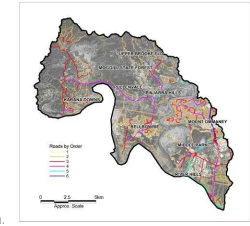
All areas discussed in this paper (with the exception of a maple leaf) are displayed in Figure 1.
Figure 1, The Study Areas
3.1.3 Additional Assessment Area Types
Based on the primary intent of this research, which was to build on what understanding there is concerning waterway networks and their relationships to their contiguous categories, additional assessment areas were assessed. This was to determine if the model derived for the estimation of waterway network relationships to themselves and their surroundings is applicable and effective in other identified natural and anthropogenic networks such as roads, leaves and pipes (see Figures 2, 3 and 4). This additional assessment was also considered to be supplementary validation for the model.
1.
Figure 2, Road Network
Figure 3, Leaf Network
Figure 4, Pipe Network
3.2 Waterways Analysis
3.2.1 SEQ Waterways Analysis
Preliminary waterway investigation involved measuring the entire lengths of SEQ waterways to associate their overall length to total catchment size. The lengths of stream ordered waterways within the catchment were then measured for verification of them being fractals, both to themselves and the total area. Using GIS, four copies (one each for area coverages of land use, rainfall, geology and slope) of the stream ordered waterway polylines were intersected and split using the attributed polygons from the areas coverage data sets. The splitting of the waterways allowed for the necessary attributes or classifications from the land use, rainfall, geology and slope layers to be augmented as attributes to the four split stream ordered waterway data sets.
Statistics from the four split, attributed SEQ waterways layers were measured and characteristics such as land use types, stream order and lengths entered into a spreadsheet. These analysis techniques were applied across the complete SEQ research region and in over 100 individual catchment and shire areas within the region. An example of one these areas is displayed in Table 3.
3.3 Pipes, Roads and Leaves Analysis
As in the Upper Oaky Creek catchment the model derived from the SEQ waterways was applied to verify if it was suitable in other areas and types of networks. The formula as described in Figure 7 was applied over pipe, road and leaf vein networks (examples of which are displayed in figures 13, 14 and 15).
4. MODEL DEVELOPMENT
4.1 Deductions to Develop New Model
Concluded from the assessment of data was that patterns and relationships form within networked data sets. The consistent theme that appeared from the data analysis was that relationships appear in all studied networks and the network objects also have relationships to the area that surrounds them. Waterway segments and lengths are fractals of themselves and the entire expanse in which they lay (Harris, McDougall et al. 2014Harris, McDougall et al. 2014). Table 1 summarises recognised relationships in waterway networks associations. Items 1 and 2 are previously identified relationships. Items 3 to 6 are derivatives from this and preceding research by the authors.
Table 1, Lengths of Waterways Relationships
1 Total length of waterways is approximately twice the area in km²
2 There are approximately two kilometres of waterways for every square kilometre area of land cover
3 For every square kilometre of land use (or land use classification) there is approximately one kilometre of stream order one waterways
4 As with land use, for every square kilometre of geology, rainfall or contiguous classifications there is approximately one kilometre of stream order one waterways
5 For every square kilometre of land use, geology and rainfall classifications there are approximately 0.5 kilometres of stream order two waterways, 0.25 kilometres of stream order 3 waterways and so on...
6 Stream order two waterways are half the length of stream order one waterways, stream order three waterways are approximately half the length of stream order two and so on...
Hence the steps within Table 2 can be applied to predict lengths of stream ordered waterways within an area or within categorisations of any contiguous area such as land use:
Table 2, Predicting Lengths of Waterways
1 Distinguish the total area size in km²
2 Double the total area (km²) in kilometres for the total length of waterways
3 Length of Stream order one waterways will be similar (in kilometres) to total area (km²)
4 Stream order 2 waterways will be approximately half stream order one and equivalent to total area number
5 Stream order 3 waterways will be half stream order 2 and so on…..
For example: Based on the initial format of the model, an area 200 km² will have approximately 400 klms of waterways. It will have 200 klms of stream order one waterways, 100 klms of stream order two and so on. If an area (km²) is identified within an region, such as categorisations of land use, the equivalent predictions can be made within each classification as they can for an entire area. Thus, if the 200 km² area had 120 km² of
remnant vegetation, 50 km² of regrowth vegetation and 30 km² of pasture the total length of waterways would be 400 klms, the waterways within remnant vegetation would be 240 klms, there would be 100 klms of waterways within the regrowth vegetation and 60 klms of waterways within the pasture area. Additionally, the pasture area would have 30 klms of stream order one waterways, 15klms of stream order two, 7.5 klms of stream order three and so on.
This knowledge allowed for the consequent phase, assessing and refining a mathematical model. The purposes for the development of the model were to suitably classify and delineate possible lengths of networks; and to suitably classify and delineate possible lengths of networks within areas surrounding them. Table 3 displays a typical output from which deductions were calculated. From these results and the information displayed in Tables 1 and 2 a basic model was developed and applied to the SEQ area (See Figure 5). This model was based on the space filling fractal dimension of 2 as identified in previous research.
Number based level of detail.
For instance for SEQ
8 orders of waterways.
A
Total Length = 45896.02
=179.98(Order 8)
28
Figure 5, Initial Formula Deducted from SEQ Data Multiplied Fractal Dimension of 2
Given a difference of over 2062 km in the predicted v the actual mapped results, refinement of the model was required. This was completed by replacing the fractal of 2 with a number derived from total length of mapped waterways divided by the total area (2.082) (As displayed in Figure 6).
=
Total Length = 47777.74 47958.4
=187.36(Order 8)
Figure 6, Refinement of Formula Deducted from Results
Figure 7 refines the method used in Figure 6 into a model. The International Archives of the Photogrammetry, Remote Sensing and Spatial Information Sciences, Volume XL-2, 2014
H
Figure 7, Model Deducted from Results
5. RESULTS
5.1 SEQ Waterway Results
The accuracy, extent and quantity of results were intended to allow for the comprehensive analysis necessary for the development of a predictive model. Results from the GIS analysis were placed in charts and spread sheets. An example of the output is displayed in Figure 8. It displays the most basic of relationships between waterways and land (or catchment area) in SEQ. Stream order one waterways being comparable to total land area and subsequent stream orders being approximately half of their preceding order.
0
Total Area and Stream Order Number
Total Area (km²) Stream Order Lengths (km)
Figure 8, SEQ Land Area - Stream Orders
The basic information presented in Figure 6 is shown with additional detail in Table 3. It details areas of land use classifications and lengths of stream ordered waterways in the respective land use, geology, rainfall and slope areas. Table 3 illustrates is indicative of the fact that even when the area classifications for land use, geology, rainfall and slope are presented in more detail, the relationships between stream ordered waterways and land use and the classifications for geology and rainfall these areas still hold. Table 3 displays the total length of waterways in the area and the total area of the overall SEQ catchment.
Table 3, SEQ - Stream Order, Land Use, Geology, Slope and Rainfall Information
Land Use Type Land Use Area (km²) 1 2 3 4 5 6 7 8 Total
Water 335.6 432.9 267.4 162.4 172.8 171.8 161.5 110.5 197 1676.3
Non Vegetated 1594.2 1164 527.9 226.8 136.7 104.4 61 57.6 11.4 2289.8
Agriculture 1574.6 1415.4 745 353.4 196.9 157.7 74.8 30 0 2973.2
Forest 10373.7 11369.5 5759.3 3171.5 1733.4 822.6 405.9 152 26.7 23440.9
Grass 8843.7 8671.8 4281.2 2145.4 1081.3 455.9 246.9 117.1 2.6 17002.2
Miscellaneous 317 303.6 147.7 76 29.4 11.2 4.7 3.1 0.3 576
Total Land Use Area (km²) 23038.8
23357.2 11728.5 6135.5 3350.5 1723.6 954.8 470.3 238 47958.4
Slope Categories % Slope Area (km²) 1 2 3 4 5 6 7 8 Total
< 10 1929.8 1596.9 795.3 389.2 309.5 276.2 222.5 168.1 208.4 1596.9
10-20 11948.3 12784.9 6504.3 3524.9 1930.3 980.3 480.7 182 26.7 26414.1
>20 9160.7 8975.4 4428.9 2221.4 1110.7 467.1 251.6 120.2 2.9 17578.2
Total Slope Area (km²) 23038.8
23357.2 11728.5 6135.5 3350.5 1723.6 954.8 470.3 238 47958.4
Geology Categories Area (km²) 1 2 3 4 5 6 7 8 Total
Metamorphic Rock 378.2 413.9 203.9 88.4 40.6 2 19.4 0 0 768.2
Unconsolidated Material 4771.8 5341.7 3703.2 2868.9 2192.1 1344.2 754.8 432.6 163.5 16801
Igneous Rock 6267.9 6144.3 2720 1110.3 434.8 120.9 61.2 0.4 0.3 10592.2
Sedimentary Rock 10316.4 10337.3 4562.7 1805.4 538.6 159.3 37.6 3.2 5.2 17449.3
Sedimentary Material 1017.7 825.6 361.4 154.3 56.4 18.8 12.2 0 0 1428.7
Water 281.5 298.4 183.1 107.7 98.2 69.3 70.7 34.3 69 930.7
Total Area of Land Use (km²) 23033.5
23361.2 11734.3 6135 3360.7 1714.5 955.9 470.5 238 47970.1
Catchment Geology Information
Total length of Waterways (km) Total length of Waterways (km)
Total length of Waterways (km)
Catchment Land Use Information
Stream Order (km)
Catchment Slope Information
Rainfall Categories (mm) Rainfall Area (km²) 1 2 3 4 5 6 7 8 Total
600 - 800 611.8 618.7 295.9 153.6 106.4 50.8 58.7 0.4 0 0
800 - 1000 10002.2 10160.3 5034.2 2522.7 1479.9 682.8 562.6 308.5 88.2 0
1000 - 1200 4207.4 4465.4 2221.8 1157.6 528.7 361.4 103.4 83 125.7 0
1200 -1400 3123.3 3182.3 1624.5 902.9 488 229.8 101 63.6 22.4 0
1400 - 1600 2317.5 2224.5 1141.6 612 330.2 171.6 61.1 0 1.6 4542.6
1600 - 1800 1806.6 1686.7 940.5 492 290 156.8 59.7 0 0 3625.7
1800 - 2000 756.7 805.7 380 239.5 118.6 52.9 9.1 15.1 0 1620.9
2000 - 2200 127.8 137.3 56.2 34.2 16.2 8.6 0 0 0 252.5
2200 - 2400 61.7 58.3 29.7 18.1 2.6 0 0 0 0 108.7
2400 - 2600 21.5 21.7 9.9 2.4 0 0 0 0 0 34
2600 - 2800 1 0.9 0.1 0 0 0 0 0 0 1
Total Area of Land Use (km²) 23037.5
23361.8 11734.4 6135 3360.6 1714.7 955.6 470.6 237.9 47970.6 Total length of Waterways (km)
Catchment Rainfall Information
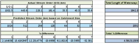
The Upper Oaky Creek catchment was used as a validation area to test the model created from analysis of the newly created data (such as that displayed in Table 3). Figures 9 and 10, along with Table 4 display further results from the Upper Oaky Creek validation.
0
Figure 9, Upper Oaky Creek – Actual v Predicted Waterways
Table 4, Upper Oaky Creek – Actual v Predicted Waterways
Total Length of Waterways
S/O 1 2 3 4 5 6 7
1002.5 443.6 228.1 161.4 33.3 40.3 33.6 1942.8
1 2 3 4 5 6 7
1024 512 256 128 64 32 16 2032
Total % Difference
1 2 3 4 5 6 7
2.144638 15.4192967 12.2314774 -20.6939 92.19219 -20.5955 -52.381 4.591311509
% Difference
Predicted Stream Order (km) based on Catchment Size Actual Stream Order (S/O) (km)
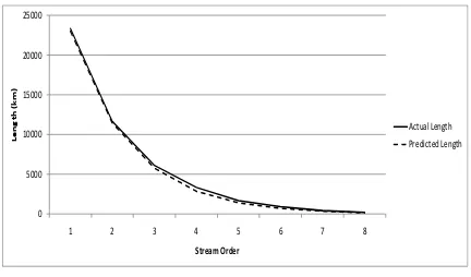
Figure 10 displays total land use areas in the Upper Oaky Creek catchment compared with predicted and ground truthed/digital stream order 1, and 2 waterways.
0
Actual Stream Order 1
Predicted Stream Order 1
Actual Stream Order 2
Predicted Stream Order 2
Linear (Actual Stream Order 1)
Linear (Predicted Stream Order 1)
Linear (Actual Stream Order 2)
Linear (Predicted Stream Order 2)
Figure 10, Upper Oaky Creek –Land Use Area v Actual Stream Order 1 and 2 Waterways, Predicted
To further test the predictive model the results were assessed in the overall 23,000 km² SEQ area. Results from the predicted and actual numbers are displayed in Figures 11 and 12, along with Table 5.
Figure 11, SEQ – Actual v Predicted Waterways
Table 5, SEQ - Actual v Predicted Waterways
1 2 3 4 5 6 7 8
23357.2 11728.5 6135.5 3350.5 1723.6 954.8 470.3 238
1 2 3 4 5 6 7 8
23038 11519 5759.5 2879.8 1440 720 360 180
1 2 3 4 5 6 7 8
-3.192 -2.095 -3.76 -4.707 -2.836 -2.348 -1.103 -0.58
Predicted Stream Order (km) based on Catchment Size
% Difference Actual stream Order (km)
Figure 12 displays total land use areas of SEQ compared with predicted and ground truthed/digital stream order 1, 2 and 3 waterways.
0 2000 4000 6000 8000 10000 12000
S
Actual Stream Order 1
Predicted Stream Order 1
Actual Stream Order 2
Predicted Stream Order 2
Linear (Actual Stream Order 1)
Linear (Predicted Stream Order 1)
Linear (Actual Stream Order 2)
Linear (Predicted Stream Order 2)
Figure 12, SEQ – Land Area v Actual Stream Order 1 and 2 Waterways, Predicted Stream Order 1 and 2 Waterways
5.2 Pipes, Roads and Leaves Results
Additional assessment of the model was applied in areas other than waterways. Both natural and anthropic areas were assessed based on the information developed in Tables 6, 7, 8 and 9.
Table 6, Moggill Creek Roads
Moggill Creek
Impervious Road Surface 1.3 12.4 10.9 6.2 7.9 7.5 44.9
Irrigated Crop and Pasture 0 0 0 0 0 0 0
Mine/Quarry 0 0 0 0 0 0 0
Native Forest 54.8 107.8 46.6 24.5 7.5 1.5 187.9
Natural Rock/Cliff 0 0 0 0 0 0 0
Non-forest Native Vegetation 0.1 0.001 0.001 0.01 0 0 0.012
Non-vegetated 2.3 5.1 3.5 1 0.7 0.4 10.7
Ocean 0.1 0 0 0 0 0 0
Plantation 0 0 0 0 0 0 0
Sand/Mud Bank 0.1 0 0 0 0 0 0
Tree Crop 0 0 0 0 0 0 0
Unclassified 0.1 0.001 0 0 0 0 0.001
Waterbody 0.1 0.1 0 0 0 0 0.1
Total Area of Land Use (km²) 66.5
146.602 68.601 34.11 17.7 9.9 276.913
Road Order
Total length of Roads (km)
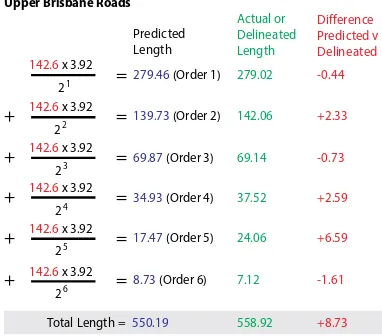
Table 7, Upper Brisbane Roads
Upper Bris. Rds.
Upper Brisbane Roads 1 2 3 4 5 6 Total 142.6 279.02 142.06 69.14 37.52 24.06 7.12 701.52
Road Order
Table 8, Maple Leaf Veins
Maple Leaf
Maple Area 1 2 3 Total
270.15 214.952 97.74 39.59 582.842
Vein Order
Table 9, Pipe Network
Pipe Size (mm) Pipe Length (m)Groupings (m)
25 2875.06
< 100 927341.92 1029492.116
150 510176.27
180 0.791
> 100 - 200 159093.75 669270.811
225 115726.76
250 16817.83
300 88036.66
375 41401.52
450 27116.84
> 200 - 500 5999.63 295099.24
525 8774.85
> 500 - 1575 16.369 135870.259
7197 2129732.426 2129732.426
5.3 Model Testing Results
The model was designed from elements of the researched data. In developing the model for network prediction, it was recognised that it needed to be as simple to use as possible. The model also needed to have the benefit of being fast, repeatable and be able to be used for multiple network types. Its structure needed to embrace and include deliberations such as the need to incorporate both network order and their relationships to their surrounding areas. The model also needed to incorporate parameters to allow it to meet the requirements of those wishing to apply it across dissimilar networks from various areas of interest. Being useable across the different networks was an important consideration. Being applicable across network types would assist substantiate and validate the model, enhancing the models reputation to accurately predict network characteristics. Results of model analysis for networks other than waterways are displayed in Figures 13, 14 and 15.
+8.73
Total Length =550.19
Predicted Length Upper Brisbane Roads
Figure 13, Upper Brisbane Road Network
+133.2 Total Length =1996.6
Predicted Length Logan Pipes
Figure 14, Logan Pipe Network
44.03 Total Length =308.25
Predicted Length Maple Leaf
Figure 15, Maple Leaf Veins Network
6. ANALYSIS AND DISCUSSION
The previous sections presented the results of the research into waterway relationships, how these results were applied to develop a model to be applied in other networks and their environments. This chapter appraises the model in the various environments and the appropriateness of the model.
The results in the previous section are of relationships between networks, in particular waterway networks are based on very large (and multiple) areas. Study over of the areas allowed for extensive statistical analysis and assessment of networks and their surroundings. Research, mostly in the SEQ region over the individual areas and types of surrounding categories, using more detailed classifications as presented in Table 3, discovered relationships between waterway networks and land areas (and categories within land) areas. The results characterised in this research are resultant from networks over large areas, allowing for a comprehensive understanding of network relationships.
Results endorse discoveries from previous works that considered relationships between networks of stream ordered waterways. Supplementary results from this research indicate that waterway relationships also occur within any recognised
land use areas. These conclusions are also applicable in areas such as rainfall and geology categories. Results displayed that data developed throughout this research indicate that network relationships occur over a variety of parameters. This includes waterway relationships to themselves and all of the coverages and classifications contiguous to them.
Furthermore, these results, being as consistent as they are over a range of landscapes and coverages become comparatively predictable. Study of the comprehensive SEQ area and additional variable areas within SEQ all indicate similar conclusions. Therefore, when the model developed in this research was applied in a new area (such as the Oaky Creek Catchment) it validated that waterway networks and individual stream order results within a variety of coverages in which they lay are predictable. The developed model could be applied to predict lengths of waterways in areas that had not beforehand been considered for assumptions to be made or are in areas of proposed modification of land use. The larger the area the more predicable these results become, but the results do apply all the way down to less significant areas such a modest 1 km² area.
Table 3 and Figures 8 and 9 demonstrate that stream ordered waterway networks measured with themselves and within catchments and classification areas over all of SEQ. Results displayed similar relationships and patterns when compared with geological areas, rainfall and flat area slope categories. Correlation analysis was used
in Figures 10 and 12 calculating the strength of association between
the numerical variables. Figures 13, 14 and 15 support the theory that the model can applied in both natural and anthropic areas.
The predictive model, when applied in a validation area such as the Upper Oaky Creek catchment (where initially only total area was known) was of significance. Using the predictive model, results relate favourably with actual lengths of stream ordered waterways. Figures 10, 11 and 12 along with Table 2 display comparisons of ground truthed and digitally generated waterway network compared with predicted lengths of waterways for the Upper Oaky Creek catchment. Figures 13, 14 and 15 and Table 5 display similar results for the SEQ area. They show a strong correlation between predicted and actual waterways within land use areas. In the Oaky Creek Catchment, ground truthed waterways have R² values of 0.9986 (stream order one) and 0.9946 (stream order two). The SEQ area presented a comparable result. Tables 4 and 5 display the percentage variance between actual and predicted lengths of waterways within the catchments. Importantly, the stream order one waterways within the network, the waterways with the most extensive overall lengths and being the crucial parts of the network that transport initial runoffs from areas, exhibit the least percentage difference.
Of note should be that real networks can display differences from the results derived from the model used in this paper. Deliberation needs to be given regarding summations made from the model, it being based on close calculations of researched networks.
6.1 Significance of Results
The significance of this work is that it will allow assessments to made without prior knowledge of networks. Subsequent to this research, some characteristics of networks can be inferred just by knowing the size of an area. For instance, we can assess how many ordered waterways will be lost in an area to be developed. We can also assess how many klms of various sized pipe networks exist under the previously developed ground and how much of a specific part of an ordered waterway network will be disturbed by changes of land use. We can assess how many waterways of a certain order have disappeared by historical development. It is important that the developed model can be applied with confidence in networks other than waterways. These networks (such as roads and pipes) add to the The International Archives of the Photogrammetry, Remote Sensing and Spatial Information Sciences, Volume XL-2, 2014
potential of the model being used in other areas whilst also assisting with its validation.
7. CONCLUSIONS
Without knowing the existing structure of anything in a comprehensive manner, it is difficult to make any kind of predictions regarding any possible characteristics. The extensively modelled and tested results in this paper demonstrate a robust propensity for relationships to exist within networked waterway lengths. Furthermore, these network relationships exist within random land areas, along with individual land use, geology and rainfall classification areas. The model developed in this work can assist with knowledge of hierarchical network assessments, assisting us understand more about existing unknown network characteristics. Lengths and relationships of networked stream ordered waterways across landscapes and environments are predictable. Outcomes from this work have extensive implications regarding how lengths of waterways within proposed development areas can be assessed. Furthermore, this same tool can be used in existing developed areas to evaluate lengths of stream ordered waterways in the area preceding any change of land use. The model will be of assistance in the future, allowing interested parties (perhaps regions where funds do not permit the creation of costly data) to ascertain more information about their networks without the necessity for the frequently challenging and expensive procedure to create this type of information digitally, particularly over large areas.
Validation of the model is its ability to be applied in networks of different types. It can be applied for assessment of various networked data sets, including things such as veins in leaves or road and pipe networks. Additional use of the predictive model may be in circumstances such as those where older cities have developed without satisfactory knowledge of underground infrastructure such as drainage, sewerage or water networks. Consideration and knowledge of asset information is important given an increased propensity to minimise capital costs. Improved knowledge of assets may enable infrastructure to be retained and kept in service for longer periods of time, or estimating its capability for growth of demand from the network. The model created in this work delivers a well trialled method for the assessment of networks. It evaluates length of hierarchy the networks, delivering results tested in both natural and anthropic environments. The model can be used for the evaluation and storage of network information such as network object categories within the contiguous area categories that surround the networks.
7.1 Moving Forward/Recommendations
Opportunities for improving the accuracy of the model exist in enabling it to more readily assess numbers of network orders (for instance there are 8 in SEQ waterways). The opportunity also exists to improve the accuracy of the model via improvements to the formula used. Both of these opportunities are being addressed as part of the ongoing research in this area. Updates will be presented in subsequent work. It is also possible that the model may also benefit from further study in areas such as predicting networks other than those studied in this work.
8. REFERENCES
Aliaga, M. and B. Gunderson (2006). Interactive Statistics, Prentice Hall.
Barthelemy, M. and A. Flammini (2008). "Modeling Urban Street Patterns." Phys. Rev. Lett 100: 1-4.
Brown, J. H., et al. (2002). "The Fractal Nature of Nature: Power Laws, Ecological Complexity and Biodiversity." The Royal Society.
Buchanan, M. (2007). "In a Different Vein." Nature Physics 3: 365.
Chappell, J. C., et al. (2012). "How Blood Vessel Networks are Made and Measured." Clells Tissues Organs(195): 94-107.
Collins (2014). Collins English Dictionary. Collins English Dictionary.
Creswell, J. W. (2007). Qualitative Inquiry and Research Design: Choosing Among Five Traditions. Califonia, Thousand Oaks, Sage Publications.
Dume, B. (2008). "City Road Networks Grow Like Biological Systems." 2014, from http://www.newscientist.com/article/dn13759-
city-road-networks-grow-like-biological-systems.html#.UxAPzPmSx8E.
Flick, U. (2009). An Introduction to Qualitative Research. Berlin, Sage Publications.
Gershenson, C. (2003) Artificial Neural Networks for Beginners. 1-3
Granger, K. and M. Lieba (2010). "The South East Queensland Setting." from http://www.ga.gov.au/image_cache/GA4202.pdf.
Harris, B. R. (2008). South East Queensland Waterways, Land Use and Slope Analysis. Engineering and Surveying. Toowoomba, University of Southern Queensland.
Harris, B. R., et al. (2014). Prediction of Waterways within Defined Areas.
La Barbera, P. L. and R. Rosso (1989). "On the Fractal Dimension of Stream Networks." Water Resources Research 25(4): 735-741.
Muijs, D. (2004). Doing Quantitative Research in Education with SPSS. London, SAGE.
Palmes, J. E. (2009). "The Origin of Valleys, a Friendly Amendment to Playfair’s Law." 2009 Portland GSA Annual Meeting: 1.
Price, C. A., et al. (2013). "The Influence of Branch Order on Optimal Leaf Vein Geometries: Murray’s Law and Area Preserving Branching." 10, from
http://www.plosone.org/article/info%3Adoi%2F10.1371%2Fjournal.p one.0085420.
Ranalli, G. and A. E. Scheideggar (1968). "Topological Significance of Stream Labelling Methods." Bulletin of the International Association of Scientific Hydrology XIII: 4-12.
Scheidegger, A. E. (1966). "Effect of Map Scale on Stream Orders." Bulletin of the International Association of Scientific Hydrology XI(3): 56-61.
Strahler, A. N. (1952). "
Hypsometric (Area Altitude) Analysis of
Erosional Topology
." The Geological Society of America 63(11):1117-1142.
Strahler, A. N. (1957). "Quantitive Anlysis of Watershed
Geomorphology." Transaction of the American Geophysical Union 38(6): 913-920.