COMPARISON OF VERY NEAR INFRARED (VNIR) WAVELENGTH FROM EO-1
HYPERION AND WORLDVIEW 2 IMAGES FOR SALTMARSH CLASSIFICATION
Sikdar M.M. Rasel a*, Hsing-Chung Chang a, Israt Jahan Diti b, Tim Ralph a, Neil Saintilan a
a Department of Environmental Sciences, Faculty of Science and Engineering, Macquarie University, NSW-2109, Australia
(sikdar.rasel, michael.chang, tim.ralph, neil.saintilan)@mq.edu.au
b Dept. of Soil Science, Faculty of Agriculture, University of Rajshahi, Rajshahi-6000, Bangladesh ([email protected])
Commission VIII, WG VIII/7
KEY WORDS: EO-1 Hyperion, Worldview 2, saltmarsh, VNIR, Wavelength, Hyperspectral, Multispectral, Classification.
ABSTRACT:
Saltmarsh is one of the important communities of wetlands. Due to a range of pressures, it has been declared as an EEC (Ecological Endangered Community) in Australia. In order to correctly identify different saltmarsh species, development of distinct spectral characteristics is essential to monitor this EEC. This research was conducted to classify saltmarsh species based on spectral characteristics in the VNIR wavelength of Hyperion Hyperspectral and Worldview 2 multispectral remote sensing data. Signal Noise Ratio (SNR) and Principal Component Analysis (PCA) were applied in Hyperion data to test data quality and to reduce data dimensionality respectively. FLAASH atmospheric correction was done to get surface reflectance data. Based on spectral and spatial information a supervised classification followed by Mapping Accuracy (%) was used to assess the classification result. SNR of Hyperion data was varied according to season and wavelength and it was higher for all land cover in VNIR wavelength. There was a significant difference between radiance and reflectance spectra. It was found that atmospheric correction improves the spectral information. Based on the PCA of 56 VNIR band of Hyperion, it was possible to segregate 16 bands that contain 99.83 % variability. Based on reference 16 bands were compared with 8 bands of Worldview 2 for classification accuracy. Overall Accuracy (OA) % for Worldview 2 was increased from 72 to 79 while for Hyperion, it was increased from 70.47 to 71.66 when bands were added orderly. Considering the significance test with z values and kappa statistics at 95% confidence level, Worldview 2 classification accuracy was higher than Hyperion data.
* Corresponding author
1. INTRODUCTION
Wetland ecosystem and their constituent components and processes are a considerable scientific interest due to their ecological function and services. Saltmarsh is an intertidal plant community dominated by herbs and low shrubs (Adam, 1996). Although Saintilan (2009) treated them not as exclusively intertidal, he defined a special characteristics that apart them from Mangrove. It has been recorded that over 40 species of fish are inhabiting in tidal saltmarsh in SE Australia alone (Daly, 2013). In addition, this ecosystems have relatively high rates of sediment carbon burial. According to Chmura (2003), globally at least 430 Tg of carbon is stored in the upper 50 cm of tidal saltmarsh soils. But this ecosystems over the world experience pressures from both human activities and natural processes that can reduce the ecosystem’s ability or capacity to recover (Goudkamp, 2006). Saintilan (2014) proved sufficient evidence that mangrove species have proliferated at least five continents over the past 50 years, at the expense of saltmarshes. Considering the current threats and pressure, this community is
treated as ‘Ecological Endangered Community’ (EEC) in
Australia (Daly, 2003). For this reasons, monitoring and dynamic change analysis of saltmarsh is a pressing issue and scientists are much more dependent on high quality remote sensing data for mapping and monitoring of wetland and their proactive management. Advanced remote sensing technology like hyperspectral data, with an ability to monitor more detailed changes in vegetation and species composition (Zomer, 2009) will expand opportunities for saltmarsh monitoring and
mapping. High spatial and spectral resolution remote sensing data with more advanced geospatial technology allows to map many changes in vegetation cover using species signature analysis. Some authors used airborne hyperspectral data, particularly, Compact Airborne Spectral Imager (CASI) imagery for mapping and monitoring salt marshes (e.g. Belluco et al. 2006; Hunter and Power 2002; Thomson et al. 2003), still the data acquisition is a time-consuming and expensive activity for airborne hyperspectral data (Hunter and Power 2002). In this respect, narrow band (198 calibrated bands) but coarse spatial resolution EO-1 Hyperion data might be an alternative. But it has a low signal to noise ratio in comparison to airborne hyperspectral sensors. The result of signal in this spacecraft lost to atmospheric absorption and the reduced energy available from surface reflectance at orbital altitude. Moreover, detector arrays used in this sensor were “spares” originally designed for another purpose, which further decreases the signal to noise ratio (Jupp & Datt, 2004). On the other hand, High Resolution Satellite Imagery (HRSI) data products are routinely evaluated during the so-called in-orbit test period, in order to verify if their quality (SNR and other radiometric properties) fits the desired features. High resolution satellite data and its recent advancement has significantly improved the coastal and saltmarsh vegetation mapping. Due to the sub-meter spatial resolution and the advantage of satellite platform for repeated data acquisition with minimal coast, Space Imagines’ IKONOS
QuickBird-2 satellite remote-sensing data Wang (2007) mapped both terrestrial and submerged aquatic vegetation communities of the National Seashore Suffolk County, New York, and achieved approximately 82% overall classification accuracy for terrestrial and 75% overall classification accuracy for submerged aquatic vegetation and provided an updated vegetation inventory and change analysis results. In another study, Ouyang (2011) used Quickbird imagery to efficiently discriminate salt-marsh monospecific vegetation stands using object-based image analysis (OBIA) classification methods in terms of accuracy than pixel-based classification method. Considering the prospect of HRSI, no mentionable research has been done using Worlview-2 for saltmarsh classification although it has finer spatial and spectral resolution compare to Quickbird. Moreover we added high spectral resolution Hyperion data to test the efficiency of spectral and spatial resolution. As the Signal-Noise-Ratio (SNR) is one of the important properties of Hyperion data, we considered this property to test the quality of the data before selecting the spectral wavelength for comparison. It was also considered the information redundancy of Hyperion data. Within 242 original bands, the information content of the one band can be fully or partially predicted from the other band in the data (Krishna, 2008). This redundancy exist due to the high correlation between bands, specially between adjacent bands ( Jiang, 2004). Hence specific algorithms like Principal Component Analysis (PCA), Minimum Noise Fraction (MNF) are generally used to remove redundant dimensions and to select optimum bands number for further analysis.
The current study explores how spectral resolution (Very Near Infrared part) and spatial resolutions of satellite images affect salt-marsh vegetation classification. For saltmarsh monitoring and management, it is essential to have a knowledge of the spatial distribution of salt-marsh vegetation types. This study focuses on the potentiality of high-spatial and high-spectral resolution satellite data for reliably salt-marsh vegetation species classification with the help of extensive ground truth data. The objectives were (1) to segregate effective number of bands from Hyperion data (2) to identify the efficiency of Visible to VNIR wavelength for saltmarsh classification from two sensors and (2) to assess the efficiency of high spatial resolution in context of coarse spectral resolution of the classes of interest. Although this study has ignored Short-Wave Infrared (SWIR) part from Hyperion, the results can then be used as a baseline information for further saltmarsh related monitoring program where spatial resolution is a fact due to small patch of species distribution.
2. STUDY AREA AND DATA SETS 2.1 Study area
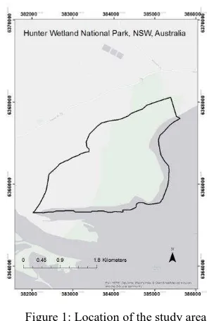
The study area is located (Longitude 151°43'40.6" E to 151°46'19.4" E and latitude 32°47'21.9" S to 32°51'29.4" S ) in Tomago, Newcastle, Australia which occurs approximately 8 km south of Raymond Terrace and 10 km north of Newcastle (NSW) (Figure 1). The study area includes the Hunter National Wetland Park and surrounding area. The topography is generally level, low lying and subject to periodical flooding. A series of drainage channels and levee banks dissect the study area.
Figure 1: Location of the study area
2.2 Remote sensing and other ancillary data
Satellite imagery from two sensors were used for this research. High-spectral resolution EO-1 Hyperion data and high-spatial resolution data from Worldview 2 and were used to compare the sensor capabilities in discriminating salt-marsh vegetation. Worldview 2 images have 0.46 m pixel resolution in the panchromatic mode and 1.84 m resolution in the multispectral mode. The multispectral mode consists of eight broad bands in the coastal blue (400-450 nm), blue (450–510 nm), Yellow (585- 625 nm), red (630-690 nm), red edge (705 – 745), NIR1 (770-895) and NIR2 (860-1040) parts of the electro-magnetic spectrum. EO-1Hyperion images have 242 narrow bands and a pixel resolution of 30 m. The Wordview-2 satellite data were captured on 5th May 2015, and the EO-1 Hyperion satellite data were captured on 6thJune, 2015.
2.3 Field data
For ground truth, an extensive fieldwork was conducted in the study area on 10th to 12th June 2015. Stratified sampling design was followed based on three strata (tree, saltmarsh and waterbody). Although homogeneity was a crucial issue for sampling size, however each of the sample sites were at least 30 m × 30 m so that the data collected could be used for the Hyperion as well as the Worldview 2 image training and classification. Sampling data included vegetation species class, percentage occurrence of each species within the selected plot and their global positioning system (GPS) locations. Total 256 sampling points and related information were recorded and divided into two parts for training and validation. 50% samples were used to train data and rest 50% were used to validate the training result. Both images were rectified using local council ( https://maps.six.nsw.gov.au/) ground control points (GCPs) to WGS 84 UTM Zone 56 S projection system. The image-processing task was carried out in ENVI Classic, ERDAS IMAGINE 2015 and ArcGIS 10.2.
2.4 Land cover and species description
3. DATA PROCESSING Processing Flow
Figure 2: Processing flow of both images. 3.1 Processing of Worldview 2 data
The radiometrically corrected Worldview 2 products are used where the pixel values are calculated as a function of the amount of spectral radiance that enters the telescope aperture and the instrument conversion of that radiation into a digital signal (Digital Globe , 2009). So it is very important to convert digital number into radiance (Figure 2) and then reflectance if we want to compare Worldview 2 data with other sensors that is related with spectral information.
3.1.1 Conversion of DN to radiance
The raw digital number (DN) has been converted to radiance data by applying the ENVI Worldview 2 calibration utility, available in ENVI v4.6 and greater. It uses the factors from the Worldview 2 metadata and applies the appropriate gains and offsets in order to convert those values to apparent radiance.
3.1.2 Atmospheric correction and surface reflectance
It is imperative that multispectral data be converted into reflectance prior to performing any spectral analysis. Currently we have top atmospheric radiance data and have to be transformed into surface reflectance data. We used FLAASH atmospheric module in ENVI classic to remove atmospheric haze and to get surface reflectance data. FLAASH Module multiply the reflectance data by 10000 to convert the heavy float type data (with decimals) into integers for fast calculations and lower data size. So, the output reflectance may exceeds 10000 (also it include negative values related to shady areas within the image where FLAASH cannot calculate the sun irradiance at it. Here we used a logical equations (Elsaid, 2014) to limit the reflectance data between 0 and 1 which is more reliable and comparable with most spectral libraries data range. Because surface reflectance is equal to Surface radiance divided by Sun irradiance. So, surface reflectance is always less than 1.
3.2 Processing of EO-1 Hyperion data
With a single scene of Hyperion observation for classification with training data, it is not necessary to use atmospherically correct image data (Datt B, 2003). Because it tends to amplify noise levels and reduces the Signal Noise Ratio (SNR). Considering our scene of wetland ecosystem we did
atmospheric correction (Figure 2) but calculated SNR well ahead with radiance data to assess data quality.
3.2.1 Elimination of bad bands based reference and other information
Among the 242 bands of L1_R Hyperion data, it has been found that some bands are set zero during level-1 processing. They are bands from 1 to 7, bands from 58 to 76 and bands from 225 to 242. The remaining 198 calibrated bands (Beck, 2003) have been used for SNR calculation. Bands 77 and 78 were removed due to low SNR ( Datt B, 2003). Water absorption bands 120 – 122, 126 -132, 165-182, 185- 187 and 221 – 224 also removed (Beck, 2003) but bands 123-125 have been retained in the image because some atmospheric correction programs like ENVI FLAASH require bands centres near 1380 nm in the strong water vapour wavelength for masking clouds. Thus 158 remaining calibrated bands used for radiometric calibration for radiance data followed by atmospheric correction.
3.2.2 SNR Calculation of EO-1 Hyperion data
EO-1 Hyperion was designed for a one-year life as test basis. But the instrument has continued to function well beyond two years with no degradation (Pearlman, 2003). It has already more than 10 years has passed and still a lot of research are in progress with this sensors. So in our work we tested SNR of 158 selected bands. After that 158 bands were radiometrically corrected in ENVI based on metadata information to get radiance data. These radiance data were used for SNR calculation. There are many analytical approach (Atkinson, 2007) to calculate SNR. The simplest way is the mean over standard deviation method by which the SNR is expressed as the ration of the mean signal over the standard deviation of a target interest. Standard approach use a 50% albedo target, however user defined targets based on interest can be selected to calculate SNR. Here SNR was calculated based on different season and different year of acquisition to find a relation with Hyperion proposed SNR.
3.2.3 Atmospheric correction
The Hyperion data has been acquired in June 2015 when there is a spectral variation in trees and shrubs was expected. FLAASH is an atmospheric correction tool that corrects wavelengths in the visible though near-infrared and shortwave infrared regions, upto 3 µm (Somdatta, 2010). The DN values of Hyperion L1_R data are scaled at-sensor radiance and stored as 16 bit signed integer that need a radiometric calibration to get the absolute radiance. Then FLAASH atmospheric correction module has been selected to convert absolute radiance values in the image to its reflectance values (ENVI User Guide).
3.2.4 Principal Component Analysis (PCA)
A spectral subset 56 bands has been selected (table 1) from 158 bands based on VNIR to SWIR wavelength (436.99 to 1043.59 nm) to match wavelength with HRSI Worldview 2 data. Hyperion is a narrow band hyperspectral data and contains redundancy of information within a narrow interval of wavelength. Principal Component Analysis (PCA) was done to produce uncorrelated bands, segregate noise components and to reduce data dimensionality of 56 bands (Table 1).
Bands Lower edges (nm)
Upper edges (nm)
Bands Wavelength (nm) range
Coastal 400 450 B9-10 436.99 – 447.17
Blue 450 510
B11-16
457.34 – 508.22
Green 510 580
B17-23
518.39 – 579.45
Yellow 585 625
B24-B27
589.62 – 620.15
Red 630 690
B28-B34
630.32 – 691.37
RedEdg 705 745
B35-B41
701.55 – 762.60
NIR1 770 895 B42-
B53
772.78-884.70
NIR2 860 1040
B64-B90
996.63-1043.59
8 Bands 56
Bands
Table 1. Band selection from both sensor.
3.3 Classification algorithm and accuracy
For supervised classification, the standard statistics “Maximum Likelihood Classifier” (MLC) algorithm was used. Overall Accuracy (OA), Producer Accuracy (PA) and User Accuracy (UA) were calculated based on confusion matrix. For the accuracy of different vegetation classes Mapping Accuracy percentage (MA %) was calculated based on the following equation (Congalaton & Green, 2008),
MA (%) = (Pixels Correctly Classified)/ (Pixels Correctly classified+ Pixels Omissions + Pixels Commissions) * 100 (1).
where
Pixels omissions is the number of pixels assigned to other classes along the row of the confusion matrix relevant to the class considered.
Pixels commissions is the number of pixels assigned to other classes along the column of the confusion matrix relevant to the class considered.
4. RESULTS
4.1 Worldview 2 data analysis and classification 4.1.1 Analysis of radiance and reflectance spectra
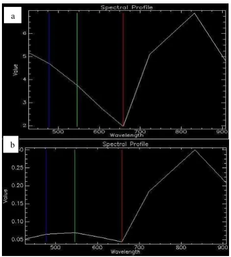
At first radiance spectrum of different vegetation and land cover classes were visually observed to check their similarity and difference with the surface reflectance spectra. The radiance spectra (figure 3a) shows high values within the blue and green part of visible wavelength due to aerosol scattering. But after
Figure 3. Radiance (a) and Surface reflectance (b) of healthy vegetation from healthy forest spectra.
FLASSH, the surface reflectance spectra (figure 3b) is corrected and blue and green values are much lower and the chlorophyll peak in the green wavelength is visible. Now this spectra is comparable with the corrected reflectance spectra of Hyperion data.
4.1.2 Classification
Arrangement of bands for classification
OA_Trai ning %
Kappa statistics
OA_V alidati on %
Kappa statistics
RGB and NIR1 97.61 0.969 72.57 0.66 RGB, NIR 1 and
Coastal
97.58 0.964 72.57 0.66
RGB, NIR1 and Yellow RGB, NIR1 and Red Edge
98.14
98.19
0.973
0.973
76.38
78.59
0.70
0.71
RGB, NIR 1 and NIR2
98.19 0.972 77.66 0.70
8 Band together 99.07 0.984 79.67 0.71
Table 2. Supervised classification of WORLDVIEW 2
It is clear from the training and validation dataset, with an increase in the number of the bands, the overall accuracy also increased except coastal band. This might be due to the absence of sea water in the study area. Over all accuracy for test site increased up to 7% with the combined 8 bands of WORLDVIEW 2 data.
a
Band Foreste for the validation classes in saltmarsh area
4.2 EO-1 Hyperion data analysis and classification
4.2.1 Signal Noise Ratio Calculation (SNR)
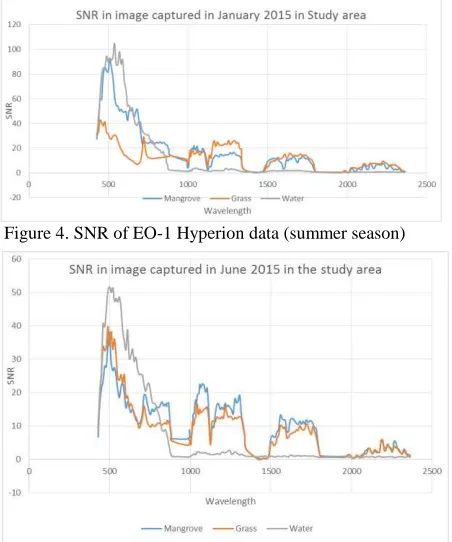
SNR varies from 0 to 110 based on the season and acquisition time. SNR is highest in VNIR region for both dataset and ranges 0 to 40 with maximum of 110 at 500 nm. Figure 4 and figure 5 shows the estimated SNR for study area in two different season.
Figure 4. SNR of EO-1 Hyperion data (summer season)
Figure 5. SNR of EO-1 Hyperion data (winter season)
The estimated SNR for both season are in good agreement with the predicted SNR for EO-1 Hyperion (Pearlman, 2003). The
SNR was one of the parameter that need to be estimated to establish the quality of images acquired by the sensors.
4.2.2 Principal Component Analysis
PCA was applied on the atmospheric corrected and spectral subset of 56 bands. Depending on the amount of information and lack of gain of variance in the increasing PCs, the initial intrinsic dimensionality is reduced to 16 components (figure 6).
Figure 6. Percentage depiction of gain in variance with increase in PCs
4.2.3 Selection of Band for classification
stress
8 Bands 16 Bands
Table 4. List of 16 selected bands for classification.
4.2.4 Analysis of Surface Reflectance Spectra
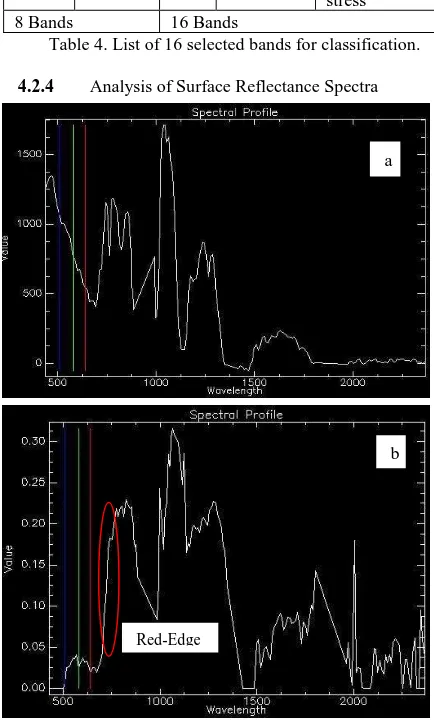
Figure 6: Radiance (a) and surface reflectance (b) spectra for healthy forest.
Radiance spectra of Hyperion data includes radiation reflected from the surface and affected by the source of radiation that is sun for optical imagery. From figure 6 (a), the radiation spectra trend toward higher values at about 500 nm, because the spectrum of the sun peaks at about 500 nm and looks like the overall shape of the solar spectrum. That is why for any quantative analysis of multispectral or hyperspectral image data, radiance image are corrected to reflectance images. From surface reflectance spectra (figure 6b), the spectra changed and red-edge part has smoothen sharply that is most important for
Table 5. Supervised classification of Hyperion data
Band Foreste the validation classes in saltmarsh area.
5. DISCUSSION
Based on 4 Hyperion scenes around the coastal region of Australia using the mean/standard deviation SNR method shows that there is a strong relationship between the acquisition time of year and the SNR of the Hyperion data. That was a good agreement with findings of Kruse (1999). Calculated SNR for Hyperion SWIR data are higher in the summer and lowest in the winter (Figure 4 and 5) that was also similar with the finding of Kruse (2003). After SNR based data quality assessment, Hyperion L1_R data were radiometrically calibrated followed by FLASSH correction.
There are clear and visible differences between radiance and reflectance spectra of Worldview 2 and EO-1 Hyperion data that becomes visible after atmospheric correction. Øystein (2012) proved that FLAASH corrected Worldview 2 image has a clearly lower blue component and expected chlorophyll peak in the green band due to the correction of aerosol scattering. In a different study conducted by Yuan (2008) showed that Hyperion image showed the rich spectral information of objects after FLAASH correction. Based on the PCA of FLAASH corrected reflectance data, only 16 bands were selected for further processing that was similar with the findings of Chauhan (2011) and Pervez (2015). From 155 atmospherically corrected band, Pervez (2015) showed that only first 10 PCs contain more than 99 % of the information. Chauhan (2011) segregated first 13 bands that contains 97 % information from 168 bands of Hyperion data. In our study, among the 56 bands of atmospherically corrected Hyperion data, 79.01% variability a
b
was contained by first PC, 96.31% variability was contained by PC2 and likewise 16 PCs contains upto 99.83% variability due to the application of PCA. PCA highlights the redundancy in data due to similar responses in some wavelength and reduce the dimensionality of data by decorrelation. When 16 selected bands of Hyperion data were compared with the 8 bands of Worldview 2 for saltmarsh classification, the overall classification accuracy has increased in both cases after adding band orderly. But the overall accuracy obtained from Worldview 2 was higher than that from EO-1 Hyperion image. Table 2 shows that OA % for Worldview 2 was increased from 72 to 79 while for Hyperion it increased from 70.47 to 71.66. Considering the significance test with z values and kappa statistics at 95% confidence level, Worldview 2 classification accuracy was higher than Hyperion data. This findings is differ from the findings of Kumar & Sinha (2014). This is might be due to the spectral properties of high spatial resolution data and ground scene of study area. Kumar and Sinha (2014) used Quick bird images that have 4 multispectral band with 2.4 m resolution. Whereas Worldview 2 images that used in our study have 1.84 m spatial resolution with 8 band in multispectral mood. Moreover they used all of the bands of Hyperion data in their study. But in our study we used only 56 Hyperion band (49 VNIR and 7 SWIR) to compare with the wavelength of Worldview 2 images. It was also segregated the number of bands to reduce the redundancy of information. Finally 16 bands based on reference were used for classification purposes.
6. CONCLUSION
This paper describes importance of SNR for data quality assessment and PCA for data reduction for EO-1 Hyperion data. Based on the VNIR of multispectral broadband and hyperspectral narrow band data this research explores the potentiality of spatial resolution over spectral resolution. Classification accuracy improved significantly in both cases after adding bands orderly. But overall accuracy was higher in case of Worldview 2 due to high spatial resolution and small patch size of species on real earth condition. The result of current study can be applied to any future research relates to SWIR for the improvement of classification accuracy. Although this research ignores the importance of SWIR, another study is on progress with SWIR of EO-1 Hyperion and Worldview-3 (8 band MSS and 8 band SWIR) data for the improvement of classification accuracy for saltmarsh species.
ACKNOWLEDGEMENTS
The author would like to greatly thank the Department of Environment and Heritage, NSW and Land and Water Division, Commonwealth Scientific and Industrial Research Organization (CSIRO), Black Mountain, ACT, Australia for data and other logistics.
REFERENCES
Adam, P., 1996. Saltmarsh. In: State of the Marine Environment Report for Australia (eds L. P. Zann & P. Kailola) pp. 97-105. Technical Annex 1. Deaprtment of Environment, Sport and Territories, Canberra.
Atkinson, P., Sargent, I., Foody, G., & Williams, J., 2007. Exploring the geostatistical method for estimating the signal-to-noise ratio of images. Photogrammetric Engineering & Remote Sensing, 73(7), 841-850.
Beck, R., 2003. EO-1 user guide, version 2.3. Satellite Systems Branch, USGS Earth Resources Observation Systems Data Center (EDC).
Belluco, E., Camuffo, M., Ferrari, S., Modenese, L., Silvestri, S., Marani, A., & Marani, M. (2006). Mapping salt-marsh vegetation by multispectral and hyperspectral remote sensing. Remote sensing of environment, 105(1), 54-67. doi:http://dx.doi.org/10.1016/j.rse.2006.06.006.
Chauhan, H. J., Mohan, B. K., & CSRE, I., 2011. Approaches to Optimum Dimensions Selection of Remotely Sensed EO-1 Hyperion Data for Crop Classification. IJCSI, 12.
Chmura, G. L., Anisfeld, S. C., Cahoon. D. R., Lynch, J. C., 2003. “Global carbon sequestration in tidal, saline wetland
soils,” Global biogeochemical cycles. 17(4), 1111.
Congalton, R. G., & Green, K., 2008. Assessing the accuracy of remotely sensed data: principles and practices: CRC press.
Datt, B., McVicar, T. R., Van Niel, T. G., Jupp, D. L., & Pearlman, J. S., 2003. Preprocessing EO-1 Hyperion hyperspectral data to support the application of agricultural indexes. Geoscience and Remote Sensing, IEEE Transactions on, 41(6), 1246-1259.
D. Globe, 2009. "DigitalGlobe Core Imagery Products Guide," D. Globe.
Daly, T., 2013 “Prime fact: Coastal Saltmarsh,” <http://www.dpi.nsw.gov.au/__data/assets/pdf_file/0007/45962 8/Coastal-Saltmarsh-Primefact.pdf> ( 17 September 2015). http://www.dpi.nsw.gov.au/
ENVI User Guide, 2003. Version 2.3.
Elsaid, M., 2014. Remote Sensing and GIS Work Station By Mahmoud Elsaid Assistant Lecturer of Geology Nuclear Materials Authority, https://www.tubeid.net/watch/download-video/5Pr0etulepH/landsat-8-data-part-i-preprocessing.html (September 14, 2015).
F.A. Kruse, J.W. Boardman, and J. F. Huntington, 2002.
“Comparison of EO-1 hyperion and airborne hyperspectral remote sensing data for geologic applications,” in Proc. SPIE Aerospace Conf., Big Sky, MO, Mar. 9–16, 2002, 6.0102, p. 12.
Goudkamp. K., Chin. A., 2006. “Mangroves and Saltmarshes
Townsville”: Great Barrier Reef Marine Park Authority.
http://www.gbrmpa.gov.au/publications/sort/mangroves_saltmar shes. (15 May 2014)
Hunter, E. L., and C. H. Power. 2002. “An Assessment of Two
Classification Methods for Mapping Thames Estuary Intertidal Habitats Using CASI Data.” International Journal of Remote Sensing23 (15): 2989–3008. doi:10.1080/01431160110075596.
Jiang, X., Tang, L., Wang, C., & Wang, C. 2004. Spectral characteristics and feature selection of hyperspectral remote sensing data. International Journal of Remote Sensing, 25(1), 51-59.
Krishna Mohan., 2008. “Hyperspectral Image Preprocessing” ISRS Pre-Symposium Tutorial on “Hyperspectral Data, Analysis Techniques and Applications”, December, 16-17, 2008, SAC, Ahmedabad.
Kruse, F., Boardman, J. W., & Huntington, J. F. (2003). Comparison of airborne hyperspectral data and EO-1 Hyperion for mineral mapping. Geoscience and Remote Sensing, IEEE Transactions on, 41(6), 1388-1400.
Kumar, L., & Sinha, P., 2014. Mapping salt-marsh land-cover vegetation using high-spatial and hyperspectral satellite data to assist wetland inventory. GIScience & Remote Sensing, 51(5), 483-497.
Ouyang, Z. T., M. Q. Zhang, X. Xie, Q. Shen, H. Q. Guo, and B. Zhao., 2011. “A Comparison of Pixel-Based and Object-Oriented Approaches to VHR Imagery for Mapping Saltmarsh
Plants. “Ecological Informatics 6: 136–146.
doi:10.1016/j.ecoinf.2011.01.002.
Øystein, R., & Øivind, D. T., 2012. Evaluation of FLAASH ATMOSPHERIC CORRECTION (220512 TropSkogTranz).
Retrieved from
https://www.nr.no/en/nrpublication?query=/file/1338298623/Ru djord-Trier_FLAASH_2012.pdf (10 Oct. 2015).
Pearlman, J. S., Barry, P. S., Segal, C. C., Shepanski, J., Beiso, D., & Carman, S. L. 2003. Hyperion, a space-based imaging spectrometer. Geoscience and Remote Sensing, IEEE Transactions on, 41(6), 1160-1173.
Pervez, W., & Khan, S., 2015. Hyperspectral Hyperion Imagery Analysis and its Application Using Spectral Analysis. ISPRS-International Archives of the Photogrammetry, Remote Sensing and Spatial Information Sciences, 1, 169-175.
Saintilan, N., 2009. Biogeography of Australian saltmarsh plants. Austral Ecology, 34(8), 929-937.
Saintilan, N., Wilson, N. C., Rogers, K., Rajkaran, A., & Krauss, K. W., 2014. Mangrove expansion and salt marsh decline at mangrove poleward limits. Global change biology, 20(1), 147-157.
Somdatta, C., & Chakrabarti, S., 2010. Preprocessing of hyperspectral data: a case study of Henry and Lothian Islands in Sunderban Region, West Bengal, India.
Thenkabail, P. S., Enclona, E. A., Ashton, M. S., & Van Der Meer, B., 2004a. Accuracy assessments of hyperspectral waveband performance for vegetation analysis applications. Remote sensing of environment, 91(3), 354-376.
Thenkabail, P. S., Enclona, E. A., Ashton, M. S., Legg, C., & De Dieu, M. J., 2004b. Hyperion, IKONOS, ALI, and ETM+ sensors in the study of African rainforests. Remote sensing of environment, 90(1), 23-43.
Thomson, A. G., R. M. Fuller, M. G. Yates, S. L. Brown, R.
Cox, and R. A.Wadsworth. 2003. “The Use of Airborne Remote
Sensing for Extensive Mapping of Intertidal Sediments and
Saltmarshes in Eastern England.” International Journal of
Remote Sensing 24 (13): 2717–2737. doi:10.1080/0143116031000066918.
Wang, Y., M. Traber, B. Milstead, and S. Stevens., 2007.
“Terrestrial and Submerged Aquatic Vegetation Mapping in
Fire Island National Seashore Using High Spatial Resolution
Remote Sensing Data.” Marine Geodesy 30 (1–2): 77–95. doi:10.1080/01490410701296226.
Yuan, J., & Niu, Z., 2008. Evaluation of atmospheric correction using FLAASH. Paper presented at the Earth Observation and Remote Sensing Applications, 2008. EORSA 2008. International Workshop on Earth Observation and Remote Sensing applications.
Zomer, R. J., Trabucco, A., Ustin, S. L., 2009. “Building spectral libraries for wetlands land cover classification and
hyperspectral remote sensing,” Journal of Environmental