FUSION OF LIDAR DATA AND MULTISPECTRAL IMAGERY FOR EFFECTIVE
BUILDING DETECTION BASED ON GRAPH AND CONNECTED COMPONENT
ANALYSIS
S. A. N. Gilania,∗, M. Awrangjebb, G. Lub
a
Faculty of Information Technology, Monash University, Australia - [email protected]
bSchool of Eng. and Info. Tech., Federation University Australia, Australia -{mohammad.awrangjeb, guojun.lu}@federation.edu.au
Commission III, WG III/1
KEY WORDS:building, detection, segmentation, LiDAR, graph, NDVI, entropy, multispectral imagery
ABSTRACT:
Building detection in complex scenes is a non-trivial exercise due to building shape variability, irregular terrain, shadows, and occlusion by highly dense vegetation. In this research, we present a graph based algorithm, which combines multispectral imagery and airborne LiDAR information to completely delineate the building boundaries in urban and densely vegetated area. In the first phase, LiDAR data is divided into two groups: ground and non-ground data, using ground height from a bare-earth DEM. A mask, known as the primary building mask, is generated from the non-ground LiDAR points where the black region represents the elevated area (buildings and trees), while the white region describes the ground (earth). The second phase begins with the process of Connected Component Analysis (CCA) where the number of objects present in the test scene are identified followed by initial boundary detection and labelling. Additionally, a graph from the connected components is generated, where each black pixel corresponds to a node. An edge of a unit distance is defined between a black pixel and a neighbouring black pixel, if any. An edge does not exist from a black pixel to a neighbouring white pixel, if any. This phenomenon produces a disconnected components graph, where each component represents a prospective building or a dense vegetation (a contiguous block of black pixels from the primary mask). In the third phase, a clustering process clusters the segmented lines, extracted from multispectral imagery, around the graph components, if possible. In the fourth step, NDVI, image entropy, and LiDAR data are utilised to discriminate between vegetation, buildings, and isolated building’s occluded parts. Finally, the initially extracted building boundary is extended pixel-wise using NDVI, entropy, and LiDAR data to completely delineate the building and to maximise the boundary reach towards building edges. The proposed technique is evaluated using two Australian data sets: Aitkenvale and Hervey Bay, for object-based and pixel-based completeness, correctness, and quality. The proposed technique detects buildings larger than 50 m2and 10 m2in the Aitkenvale site with 100% and 91% accuracy, respectively, while in the Hervey Bay site it performs better with 100% accuracy for buildings larger than 10 m2
in area.
1. INTRODUCTION
The building detection from remotely sensed data has become a topic of increasing importance as they are essential for a vari-ety of applications in residential and urban areas. Their accurate boundaries are indispensable and significant for applications in the field of real estate, city planning, disaster management, carto-graphic mapping and civilian and military emergency responses (Sohn and Dowman, 2007, Li and Wu, 2013). The automatic boundary extraction is challenging due to building shape vari-ability and surrounding environment complexity. High resolution imagery contains rich spectral information that is suspectable to noise and can easily be affected by contrast, illumination, and occlusion. Under certain conditions, similar objects may appear with varying spectral signatures while different objects may pro-vide co-spectral signatures (Li and Wu, 2013).
The airborne Light Detection and Ranging (LiDAR) can rapidly acquire high-precision three-dimensional information of large-scale areas by emitting and receiving the laser pulses. The height variation is a more suitable cue for detecting elevated objects and delineating building boundaries more than the spectral and tex-ture changes. However, the horizontal accuracy of boundaries extracted from LiDAR data is poor, which makes detection more difficult (Chen and Zhao, 2012, Li and Wu, 2013). The urban areas that are characterised by complex scenes, the appearances
∗Corresponding authors: [email protected]
of trees and buildings in the LiDAR data might be similar (Rot-tensteiner et al., 2005). The combination of these two paradigms promises to produce results at greater accuracy than the contri-butions of either field alone. Therefore, many researchers have been attempting to integrate multi-source data to detect buildings in urban areas.
According to Lee et al. (Lee et al., 2008), building detection ap-proaches can be broadly categorised into three distinct groups. The first group contains methods that employ only 2D or 3D in-formation from photogrammetric imagery to detect buildings and discern from surrounding objects (Mayer, 1999). The complexity of these techniques increases proportionally with the increase in richness of information in high-resolution imagery, e.g. deriva-tion of depth informaderiva-tion from stereo to effectively address oc-clusion and shadow factors (Yong and Huayi, 2008). In addition, nearby trees of similar height also make the use of such derived range data difficult (Lee et al., 2008).
accuracy of boundaries extracted from LiDAR data is poor be-cause of laser pulse discontinuity (Li and Wu, 2013) and hard to obtain geometrically precise boundary using only LiDAR points cloud (Yong and Huayi, 2008). The quality of regularised build-ing boundaries also depends on LiDAR resolution (Sampath and Shan, 2007).
LiDAR generally provides more accurate height information but lacks in horizontal accuracy whereas high-resolution imagery en-tails precise horizontal accuracy. The third category of meth-ods exploits the complementary benefits of both LiDAR data and photogrammetric imagery. More specifically, laser intensity and height information in LiDAR data can be used along with texture and region boundary information extracted from aerial imagery to improve detection accuracy (Lee et al., 2008). As a result, several authors promoted the fusion of two data sources as a promising strategy to extract high quality building boundaries (Rottensteiner et al., 2005, Yong and Huayi, 2008, Demir et al., 2009, Li and Wu, 2013).
However, it is still challenging to extract the correct and rele-vant features from multispectral image and LiDAR data of a par-ticular area to detect buildings. But how to amalgamate the re-spective data sources such that their weaknesses can be compen-sated effectively is a question that requires further investigation. Additionally, there is no rule of thumb to integrate different fea-tures for automatic building boundary extraction of various build-ing shapes: curved, wavy, zigzag, and other irregular structures. Most existing fusion methods can only handle simple building shapes like polygons (Yong and Huayi, 2008, Awrangjeb et al., 2010).
Currently, there are no unanimous evaluation system and standard guidelines available to measure the performance of building ex-traction techniques (Rutzinger et al., 2009, Awrangjeb and Fraser, 2014a). Indeed, evaluation results are often missing from pub-lished accounts of building detection; the use of 1–2 evaluation indices only has characterised many studies (Demir et al., 2009, Awrangjeb et al., 2010). This research aims to develop, firstly, a mechanism to effectively integrate features extracted from Li-DAR and multispectral imagery to increase building detection performance and, secondly, a comprehensive evaluation of the proposed method using an automatic performance evaluation sys-tem using 15 evaluation indices (Awrangjeb and Fraser, 2014a).
In order to automatically detect buildings from complex geographic environment and delineate the boundaries, a new method is pro-posed that integrates both airborne LiDAR and multispectral im-agery. The raw LiDAR data is divided into ground data and non-ground data based on height information from bare-earth DEM and create a primary building mask. All the strongly connected pixels, the black pixels, present in the primary building mask are cumulated into contiguous regions that are later processed to es-timate initial boundary and component labelling. The resultant information is further utilised to construct a disconnected com-ponents graph where each subgraph corresponds to a contiguous region of black pixels. The resultant disconnected graph may contain heaps of subgraphs due to the fact that even a single iso-lated black pixel from primary mask become a subgraph with one node. The subgraphs identified by this process along with respec-tive boundaries and labels are further processed.
The image lines are extracted and classified using (Awrangjeb et al., 2013) and fed into a graph-based clustering procedure. The clustering process aims to associate the line segments to the cor-responding subgraph using Dijkstra algorithm. The subgraphs that fail to cluster any line are eliminated for subsequent pro-cessing and, thus, reduce the initial count of prospective build-ing objects. In order to eliminate vegetation and detect buildbuild-ing
objects, the input image is segmented into homogeneous grids and then individual cells are accumulated based on NDVI, en-tropy, and height difference. This process detects building ob-jects, separates the occluded building parts from vegetation, and estimate the respective boundary. Finally, the building boundary is expanded, if possible, by accumulating the pixels based on its NDVI, entropy, and neighbouring LiDAR points cloud. It is ex-perimentally demonstrated that the proposed technique can detect polyhedral buildings with a favourable success rate. We achieved above 90% detection rate in densely vegetated Australian urban environments whereas 100% in a low vegetation area.
The involved automatic evaluation system employs both object-and pixel-based indices. Although pixel-based evaluation reflects the horizontal accuracy, but the geometric evaluation is also used as a means of direct estimation of geometric accuracy.
2. RELATED WORK
The integration of high-resolution imagery and LiDAR data is well appreciated as it yields complementary benefits by providing a more complete scene description enriched with both spectral and 3D surface information. This integration of both data sources has been exploited to increase the classification performance and to improve the accuracy and robustness in automatic building de-tection, reconstruction and change detection techniques (Awrang-jeb et al., 2010, Awrang(Awrang-jeb et al., 2012, Li and Wu, 2013).
These integration techniques can be categorised into two subse-quent groups. Firstly, the integration techniques reported in lit-erature (Sohn and Dowman, 2007, Lee et al., 2008, Demir et al., 2009, Awrangjeb et al., 2010, Awrangjeb et al., 2012, Chen and Zhao, 2012, Awrangjeb et al., 2013, Li and Wu, 2013) utilise both the LiDAR data and the imagery as the primary cues to delin-eate building outlines. They also employ the imagery to extract features like NDVI, entropy, shadow, and illumination in order to eliminate vegetation. Consequently, they offer better horizon-tal accuracy for the detected buildings. Our proposed building detection technique falls under this group. (Rottensteiner et al., 2003) generates two digital surface models (DSMs) from the first and last pulse return of the LiDAR data, which are used along with NDVI for the detection process. A morphological filter is applied over the last pulse DSM to generate a digital terrain model (DTM). The initial building regions are identified based on height, size, NDVI and the difference between the first and last phase of the DSMs.
followed by building boundary. Vegetation is removed using fea-tures such as NDVI, entropy and height information from optical image and LiDAR data.
Secondly, there are techniques, which use the LiDAR data as the primary cue for building detection and use the features from op-tical imagery only to remove vegetation (Vu et al., 2009, Rotten-steiner et al., 2005). Consequently, these methods suffer from poor horizontal accuracy for the building boundary delineation. The method details in (Rottensteiner et al., 2005) uses the Demp-ster–Shafer theory to classify LiDAR data points into constituent groups: buildings, trees, grassland or bare soil. However, the reported detection performance is adversely affected for small sized buildings (Rottensteiner et al., 2007). The reason lies if the Dempster–Shafer model remains untrained, the misclassifica-tion rate increases considerably (Khoshelham et al., 2008). Vu et al. (Vu et al., 2009) uses a morphological scale space for extract-ing buildextract-ing footprints from the elevation data and then remove vegetation using the spectral information. The detection perfor-mance was low and high computational complexity was reported because of using the scale space.
The method presented in this research is fully data-driven and self-adaptive for diverse building shapes. This paper is organised as follows. The work flow and detailed procedure of the proposed method is provided in Section 3. The evaluation system and ex-perimental results are described and discussed in Section 4. Fi-nally, the conclusion and future research direction are provided in Section 5.
3. PROPOSED METHODOLOGY
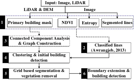
The work flow of the proposed method is shown in Figure 1. The labels from 1-6 describe the order of sub-processes towards build-ing boundary delineation. The first step, blue coloured dashed rectangle, is a data preprocessing phase where we separate Li-DAR points cloud, generate DEM, compute image entropy, NDVI and extract image line segments. The proposed method first di-vides the input LiDAR data into ground and non-ground points. The non-ground points, representing elevated objects above the ground such as buildings and trees, are further processed for build-ing detection.
NDVI Segmented lines
Image LiDAR & DEM
Input: Image, LiDAR
Primary building mask Entropy
Connected Component Analysis & Graph Construction
3
Clustering & initial building detection
4
Grid based segmentation & vegetation removal
5 Boundary extension &
building detection
6 1
Classified lines (Awrangjeb, 2013)
2
Figure 1. Work flow of proposed building detection technique
During the second phase, the extracted image lines are classi-fied into several classes e.g. ground, ridge, and edge. The line segments that belong to ‘edge‘ and ‘ridge‘ classes are of interest because these lines are either close or fall within the area of ele-vated objects. The next phase begins with Connected Component Analysis (CCA) and graph construction, where all the strongly
connected pixels from the primary building mask are collected into individual components followed by initial boundary extrac-tion. Moreover, we construct a disconnected components graph from connected components that clusters the classified lines to their particular components. We employ Dijkstra shortest path algorithm to establish the relevance of a segmented line to its corresponding component extracted from the primary building mask. The connected components that fail to cluster any line during clustering process are eliminated for further investigation, which reduces actual objects found at the first place.
We establish from literature that average height difference be-tween neighbouring LiDAR points on building rooftops change constantly but on trees, height variation is abrupt and changes variably. Moreover, the NDVI and entropy measures are rela-tively high on vegetation than building roofs (Awrangjeb et al., 2013). Therefore, to eliminate the vegetation and detect build-ings, which may partly occluded or non-occluded, the multispec-tral image is divided into equi-sized grids. The grid cells are accu-mulated under certain criteria for detection and elimination pur-poses. The grid-based segmentation process detects the buildings and estimate their corresponding boundaries. The boundary of detected buildings are finely delineated but are much shrinker due to misregistration between LiDAR and corresponding multispec-tral image. Therefore, the obtained boundaries are processed and are expanded, if possible, to extend its coverage towards building edges by accumulating individual pixels based on NDVI, entropy, and LiDAR data.
The input image in Figure 2(a) is an urban site, Aitkenvale (AV), in Queensland Australia that covers an area of214mx159m
and contains 63 buildings. In the following subsections, different steps of the proposed method are described using this scene.
(a) (b) (c)
Figure 2. Sample data: (a) Aitkenvale multispectral image, (b) Primary building mask, and (c) CCA output with initial boundary and labels
3.1 DATA PREPROCESSING AND LINE SEGMENTATION
We generate a bare-earth DEM with 1m resolution from input Li-DAR data. The bare-earth DEM is also named as Digital Terrain Model (DTM) but we refer as DEM. A primary building mask is generated, see Figure 2(b), using LiDAR data and height informa-tion from DEM according to the method reported in (Awrangjeb et al., 2010). A height threshold is computed for each LiDAR point asHt=Hg+Hrf, whereHgis ground height andHrfis a relief factor that separates low objects from higher objects. For our study, we choose 1m relief factor in order to keep low height objects (Awrangjeb and Fraser, 2014b).
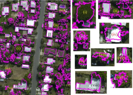
available, then the pseudo-NDVI is calculated from a colour or-thoimage (Awrangjeb et al., 2013). The texture information like entropy is estimated at each image pixel location using a grey-scale version of the image(Gonzalez et al., 2003). In step 2 of Fig-ure 1, the same grey-scale image is used to extract line segments, which are classified into several groups: ground, edge, and ridge lines, using the reported method in (Awrangjeb et al., 2013). The classification of line segments into groups is performed based on NDVI, entropy, and primary building mask computed in preced-ing phase. The segmented lines that belong to ‘edge‘ and ‘ridge‘ classes are displayed in Figure 3(c).
(a) (b) (c)
Figure 3. (a) Building boundaries detected after CCA, (b) False boundary delineation, and (c) Segmented lines (edges and ridges)
3.2 INITIAL DETECTION USING CONNECTED COM-PONENT ANALYSIS AND GRAPH TECHNIQUE
A connected component of valueυis a set of pixelsξwhere each pixel having a valueυ, such that every pair of pixels in the setφ
are connected with respect toυ. Provided that the primary mask in Figure 2(b) is a binary image that contains only two colours: black and white, where black regions describe the elevated ar-eas. So,P(r, c)=P(r′, c′)=υwhere eitherυ=blackorυ=
white. The pixel(r, c)is connected to the pixel(r0, c0)in 8-neighbourhood connectivity with respect to valueυif there is a sequence of black pixels(r, c)=(r0, c0),(r1, c1). . .(rn, cn) =
(r0, c0)whereP(ri, ci)=υ; i =0. . . n,and(ri, ci)neighbours
(ri−1, ci−1)for each i =1. . . n. The sequence of pixels(r0, c0). . .(rn, cn) forms a connected path from(r, c)to(r0, c0).
The CCA process detected 936 different objects from the primary building mask. Subsequently, we also estimated the boundary of each component using theMoore-Neighborhood tracing
algorithm. The output of CCA process is shown in Figure 2(c),
where the detected objects are labelled and plotted with different colours as of their neighbours. To visually inspect the building outline accuracy, the estimated boundaries are shown in Figure 3(a). We can clearly notice that few buildings are well delineated but several regions are formed on trees due to elevation. We can further observe that various buildings are occluded partly or fully by nearby vegetation. Moreover, some buildings are connected to each other by dense vegetation giving an indication of a single object. The building objects displayed in Figure 3(b) from (i)-(vii) describe some such situations.
So, we use the segmented lines as a feature of structural objects to eliminate the false components formed on vegetation. The lines on vegetation are differentiable because they are discontinuous, smaller, and does not establish any geometric relationship - par-allel, perpendicular, or diagonal relationship. Furthermore, we use ‘edge‘ and ‘ridge‘ lines because they are either close to the boundary or fall completely within the boundary of a particular object. In order to establish the relationship among lines and the association with their corresponding objects, we construct a
bidirectional disconnected components graph, where each con-nected component from the preceding stage is represented as a subgraph. Each pixel of an object corresponds to a node where its 8-neighbouring pixels become its child nodes. The edge from a node to its descendent is assigned a unit weight. On the contrary, there is no path between black-pixel to white-pixel and vice versa. Therefore, no edge/path is represented by ‘inf‘ edge weight to differentiate between valid and invalid paths.
The image lines clustering process begins with the selection of a longest ‘ridge‘ line as acentroidthat falls within the bound-ary of a particular object. Then, we compute the shortest dis-tance between centroid and surrounding lines usingDijkstra algorithm. The situation when the candidate line is along or on a particular shape/object, we always obtain a valid path of some weight otherwise the path weight is infinite indicating that the candidate line does not belong to the current cluster. We continue this process until all objects detected from the primary building mask are processed. The objects that fail to cluster any line are eliminated for further investigation. In this case, many objects that are formed on trees due to few LiDAR points are success-fully removed and the number of total potential objects decreased to 307 from an initial count of 936.
3.3 VEGETATION REMOVAL AND BOUNDARY DELIN-EATION
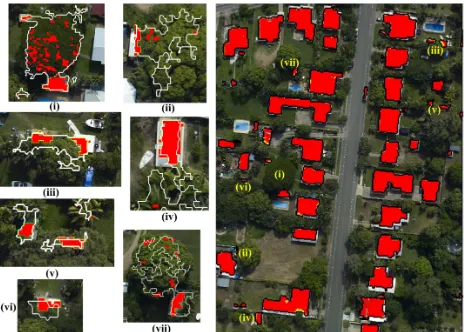
A visual comparison between Figure 3(a) and 4(a) reveals that clustering procedure drastically reduces the number of objects identified previously without losing any potential objects includ-ing small and low height buildinclud-ings. But still it is observable that heaps of false objects/boundaries exist on trees and even outline of large buildings are not properly delineated. We can further no-tice in Figure 4(a) labelled from (i) to (ix) and their corresponding zoomed version in Figure 4(b) that there are various buildings, which are heavily occluded by dense vegetation.
Figure 4. (a) Building after clustering process, (b) Occluded and false delineated buildings
the grid size. The grid size is chosen keeping the fact that each grid cell must contain LiDAR points. For example, in case of AV data set, LiDAR point density is 29 points/m2 that allows to choose a fairly smaller grid size of25cm. Therefore, the test scene is divided into rows and columns of the selected grid size.
It is quite evident from Figure 4(a) that the building objects iden-tified are not well delineated, boundaries are over-segmented and, in few cases, see (i)-(iii) and (vi) in Figure 4(b), the prospec-tive building objects are heavily occluded, and are mutually con-nected. To cope with the issues surfaced, each identified object is processed separately for vegetation removal, building recovery, and its respective boundary delineation.
Firstly, the coarse boundary associated with an object is utilised to collect the grid cells that creates a stack. Then a cell from top of the stack is selected, called seed cell, followed by the selection of cells in its 8-neighbourhood. Each neighbouring individual cell that exhibits similar height difference, NDVI, and entropy value with respect to the seed cell is accumulated, and thus, forms a group. The seed and its neighbouring cells, which meet the con-dition, are removed from the stack, and pushed into a priority queue. The seed element is marked to avoid for further selec-tion and a new seed cell is chosen from the queue followed by its neighbourhood from the stack. All candidate cells are again evaluated for different matrices: height difference, NDVI, and en-tropy, and later pushed into the queue. This cell-based segmenta-tion process continues until the last cell remains in the stack. The cells, which fail to form a group are eliminated during execution.
This process engenders contiguous groups of cells that are formed within the object’s boundary as shown in sub-figures labelled (i)-(vii) in Figure 5(a). It can be seen in the top left image labelled (i) that cell-based segmentation process has formed several groups, among all, two groups are formed on real building objects. Fi-nally, a rule-based procedure is adopted that is based on LiDAR points height difference, NDVI, and entropy, the cumulated cells, which are confined within the boundary, are eliminated and two occluded buildings are recovered. The final detected buildings and their corresponding boundaries are shown ‘yellow‘ in colour filled with red, while the groups/clusters marked for elimination have no boundary around.
Figure 5. (a) Vegetation removal and recovery of occluded build-ings, (b) Detected buildings
The same operation is performed for all the building objects ex-tracted from the last phase. It can be observed in Figure 5(a), all buildings labelled from (ii) to (vii) are well delineated and cover the actual building region. The outcome of this procedure can be
seen in Figure 5(b), where false buildings have been removed, oc-cluded buildings are recovered and building boundaries are well delineated.
(a) (b)
Figure 6. (a) Buildings before boundary expansion, (b) Final de-tected buildings
The boundaries of finally detected buildings in Figure 5(b) and Figure 6(a) are well outlined but they sometimes lack in a com-plete rooftop coverage due to large grid size as compared to the image resolution. Similar to the grid-based segmentation process, we accumulate pixels into boundary instead of cells and grow the boundary region towards edges for accurate delineation of the building boundary. For pixel based extension procedure, we first determine all the corresponding pixels of a building bound-ary and grow the boundbound-ary pixels in 8-neighbourhood fashion. For all new pixels, which does not lie within the already estab-lished boundary, we compute the pixel NDVI and height of their respective LiDAR data points. The pixel is included as a new boundary pixel based on comparison with average NDVI of pix-els and LiDAR points average height within the boundary. Sim-ilarly, rest of the boundary pixels including new pixels, if any, are processed. We repeat the same process for all the buildings. The pre-expansion and post-expansion boundaries can be seen in Figure 6(a) and Figure 6(b) respectively. The later figure shows the final building boundaries that cover the building rooftop well close towards the building edges and will be used for evaluation purpose.
4. EXPERIMENTAL RESULTS AND DISCUSSION
To evaluate the performance of the proposed approach, two test data sets from two different sites are used. The objective eval-uation follows a modified version of a previous automatic and threshold-free evaluation system (Awrangjeb and Fraser, 2014a).
4.1 DATA SETS
The test data sets as shown in Figure 7 cover two urban areas in Queensland, Australia: Aitkenvale (AV) and Hervey Bay (HB). The AV data set has a point density of 29 points/m2 and com-prises of a scene that covers an area of214mx159m. This scene contains 63 buildings, out of those four are between 4 to 5m2
and ten are between 5 to 10m2
(a) (b)
Figure 7. Data sets with reference boundary: (a) Aitkenvale, (b) Hervey Bay
4.2 EVALUATION SYSTEM
In order to assess the performance of the proposed method, the automatic and threshold-free evaluation system (Awrangjeb and Fraser, 2014a) has been employed. It offers more robust object-based evaluation of building extraction techniques than the threshold-based system (Rutzinger et al., 2009) adopted by the ISPRS bench-mark system. It makes one-to-one correspondences between de-tected and reference buildings using the maximum overlaps, es-timated by number of pixels. If a reference buildingrr and a detected buildingrdoverlaps each other and they do not overlap any other entities, a true-positive (TP) correspondence is simply established. If a detected buildingrd does not overlap anyrr, then it is marked as a false positive (FP). Similarly, if a refer-ence buildingrrdoes not overlap anyrd, then it is marked as a false negative (FN). In any other cases, anrdoverlaps more than onerrand/or anrroverlaps more thanrd. In these two cases, a topological clarification is executed to merge or split the detected entities.
The reference data sets overlaid on the two test data sets, as shown in Figure 7, are used. The objective evaluation uses different eval-uation metrics for three different types of evaleval-uation categories: object-based, pixel-based, and geometric. For object-based met-rics, completeness, correctness, quality, under- and over-segmentation errors give an estimation of the performance by counting the num-ber of detected objects in the study. Whereas pixel-based metrics such as completeness, correctness and quality measures deter-mine the accuracy of the extracted objects by counting the num-ber of pixels. In addition, the geometric metric, root mean square error (RMSE), indicate the accuracy of the extracted boundaries with respect to the reference entities. Moreover, the number of over- and under-segmentation cases are estimated by the num-ber of split and merge operations required during the topological clarification.
The minimum areas for large buildings and small buildings have been set to50m2
and10m2
, respectively, in Awrangjeb and Fraser (Awrangjeb and Fraser, 2014b). Thus, the object-based complete-ness, correctness and quality values will be separately shown for large buildings and small buildings.
4.3 EVALUATION RESULTS
Figures 8 and 9 show the extracted buildings for the AV and HB data sets. The preceding figure also shows some complex cases, where the proposed method has not only detected small build-ings but has also recovered the occluded buildbuild-ings successfully.
(a)
(b) (c)
(d) (e) (f)
(h) (i)
(k) (l)
(n)
(o)
(g)
(j)
(m)
Building missed! Building detected
Under extension
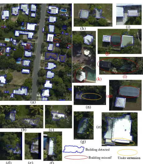
Figure 8. (a) Building detection on AV data set, (b)-(g) Magni-fied version of the buildings detected under complex scene, (h)-(i) Boundary over-extension, (j)-(m) Undetected buildings, (n)-(p) Boundary under-extension
For quantitative analysis of proposed method, object-based eval-uation results are presented in Table 1, while pixel-based and ge-ometric evaluation results are given in Table 2, respectively.
(a) (b)
(d) (c)
Figure 9. (a) Hervey Bay reference data set, (b) Detected build-ings
The proposed technique is equally effective in both test areas. If we consider all reference buildings irrespective of their areas, the average completeness and correctness in object-based evalu-ation is above 92% with an average quality of about 92% (Table 1). All the buildings detected from Aitkenvale test scene can be seen in Figure 8(a). The magnified figures from (b) to (g) show some complex cases, where buildings are completely occluded by nearby dense vegetation. Two such buildings can be observed in Figure 9(b). Building (d) is of equal height of the surrounded vegetation and building (c) is close enough to a large building.
Areas Cm Cr Ql Cm,50 Cr,50 Q1,50 Cm,10 Cr,10 Q1,10
AV 84.62 100 84.62 100 100 100 91.67 100 91.67
HB 100 100 100 100 100 100 100 100 100
Avg 92.31 100 92.31 100 100 100 95.83 100 95.83
Table 1. Building detection results: object-based evaluation for the Aitkenvale(AV)and Hervey Bay(HB)data sets in percentage.
Cm= completeness,Cr= correctness andQl= quality, are for buildings of50m
2
and10m2
Areas Cmp Crp Qlp Aoe Ace RM SE Cm,50 Cr,50 Cm,10 Cr,10
AV 88.85 96.71 86.25 11.14 3.28 0.58 91.0 96.71 89.32 96.71
HB 86.95 96.72 84.45 13.0 3.28 1.18 86.95 96.71 86.95 96.71
Avg 87.90 96.72 85.35 12.07 3.28 0.8 88.97 96.71 88.14 96.71
Table 2. Building detection results: pixel-based evaluation for the Aitkenvale(AV)and Hervey Bay(HB)data sets in percentage.
Cmp= completeness,Crp= correctness andQlp= quality,Aoe= area omission error andAce= area commission error in percentage,
RM SE= planimetric accuracy in metres
segmentation (last step), the NDVI value and average height of LiDAR points in that particular region, were laying well within the rule window that caused boundary to extend on tree bush and ground for buildings (h) and (i) respectively. The similar phe-nomenon can be observed from Figure (d) in 9(b), where part of bush was also included into the boundary due to similar height of building.
The buildings encircled with red ovals in Figure 8 (j)-(m) were not detected due to transparent roof material. These buildings have also been marked to their corresponding positions in Figure 8(a). These buildings were eliminated while generating primary building mask in first step because there were not LiDAR returns recorded for these buildings. But small sized umbrella (k) was missed due to extremely small sized and misalignment between both input data sources. The buildings (n) and (o), marked with ‘yellow‘ coloured oval in Figure 8(a), are the cases where build-ing boundaries were not expanded towards buildbuild-ing edges. The reason that actually stopped the boundary extension procedure in case of building (n) was a variation in LiDAR data height in the neighbourhood due to nearby vegetation. But the building (o) suffered merely because of misalignment between two data sources.
It is quite evident from Table 1 that the proposed technique has not only detected buildings larger than50m2
with100% accu-racy but has also extracted low height buildings with equal ac-curacy. As further can be noticed from Table 2, which tabu-lates pixel-based evaluation results, the average completeness, and quality values are even2 to 4% higher than those in the object-based evaluation for the AV site. It can further be seen that our proposed algorithm offers an average accuracy of about 89%and96%in pixel-based completeness and correctness for buildings larger than50m2
, while at the same it gives an average accuracy of around88%and96% in pixel-based completeness and correctness for buildings smaller than10m2
respectively.
4.4 COMPARATIVE PERFORMANCE
The method proposed in this research outperforms the algorithm reported in (Awrangjeb and Fraser, 2014b) in completeness and correctness for both object-based and pixel-based evaluation. For the AV site, our proposed algorithm showed significantly better object-based accuracy than (Awrangjeb and Fraser, 2014b)–91% vs 67%, for the buildings smaller than10m2
. Similarly, in terms of pixel-based accuracy, our proposed method offers88%as com-pared to 86% of Awrangjeb’s technique when all building objects are considered.
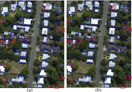
The visual comparative results of both detection techniques re-ported in (Awrangjeb and Fraser, 2014b) and proposed algorithm
are shown in Figure 10 (a) and (b) respectively. We can clearly observe that Awrangjeb’s algorithm fails to detect 11 buildings highlighted in red colour whereas the corresponding buildings de-tected by our proposed algorithm are shown in 10(b). Addition-ally, it can be noticed from building marked by yellow coloured oval in 10(a) that Awrangjeb’s method fails to completely delin-eate the building, thus, indicate under-segmentation issue. But the corresponding yellow coloured oval in 10(b) shows that the proposed algorithm can successfully delineate the extended build-ing parts efficiently.
But in case of the HB site, both the algorithms offer the same object-based accuracy for larger buildings. However, the pixel-based completeness of the proposed technique is 96% as of 93% by (Awrangjeb and Fraser, 2014b) for buildings larger than50m2
.
(b) (a)
Figure 10. (a) Buildings missed by Awrangjeb(2014) detection technique, (b) Building detection result of proposed method
5. CONCLUSION
The automatic extraction of accurate building boundaries is an important geo-spatial information that is indispensable for several applications. The most challenging factor confronted in boundary delineation is building shape variability and surrounding environ-ment complexity. In order to deal with various building types, this research presents a new method for automatic building detection through an effective integration of LiDAR data and multispectral imagery.
carried on primary building mask, derived from LiDAR data. Later on, several building features are extracted from multispec-tral image that are progressively used in different stages to elim-inate false objects and vegetation, detect buildings, and delineate the corresponding building boundaries.
The final building boundary is obtained by extending the initial position using both the data sources: features extracted from im-age and LiDAR data. The whole procedure imposes no constraint on building shape variability and surrounding environment. This method is fully data-driven, self-adaptive and avoids the under-segmentation and over-under-segmentation issues. The proposed method is not only capable of detecting small buildings, but can also sep-arate the buildings from surrounding dense vegetation and close buildings.
In future, the segmented lines extracted from multispectral im-agery will be incorporated to obtain better planimetric accuracy and to generate the building footprints. This would help to de-velop 2D representation and reconstruction of roof features (e.g. roof planes, chimneys, and dorms) with the integration of LiDAR data. The accuracy and performance of the proposed approach will further be analysed on ISPRS benchmark data sets with dif-ferent LiDAR resolutions.
ACKNOWLEDGEMENTS
The research is supported under the Discovery Early Career Re-searcher Award by the Australian Research Council (project num-ber DE120101778). The Aitkenvale and Hervey Bay data sets were provided by Ergon Energy (http://www.ergon.com.au) in Queensland, Australia.
REFERENCES
Awrangjeb, M. and Fraser, C., 2014a. An automatic and threshold-free performance evaluation system for building ex-traction techniques from airborne lidar data. Selected Topics in Applied Earth Observations and Remote Sensing, IEEE Journal of 7(10), pp. 4184–4198.
Awrangjeb, M. and Fraser, C. S., 2014b. Automatic segmentation of raw lidar data for extraction of building roofs. Remote Sensing 6(5), pp. 3716–3751.
Awrangjeb, M., Ravanbakhsh, M. and Fraser, C. S., 2010. Auto-matic detection of residential buildings using lidar data and multi-spectral imagery. ISPRS Journal of Photogrammetry and Remote Sensing 65(5), pp. 457–467.
Awrangjeb, M., Zhang, C. and Fraser, C. S., 2012. Building de-tection in complex scenes thorough effective separation of build-ings from trees. Photogrammetric Engineering & Remote Sens-ing 78(7), pp. 729–745.
Awrangjeb, M., Zhang, C. and Fraser, C. S., 2013. Automatic extraction of building roofs using lidar data and multispectral im-agery. ISPRS Journal of Photogrammetry and Remote Sensing 83(9), pp. 1–18.
Chen, L. and Zhao, S., 2012. Building detection in an urban area using lidar data and quickbird imagery. International Journal of Remote Sensing 33(15), pp. 5135–5148.
Demir, N., Poli, D. and Baltsavias, E., 2009. Extraction of build-ings using images & lidar data and a combination of various methods. International Archives of the Photogrammetry, Remote Sensing and Spatial Information Sciences 38(part 3/W4), pp. 71– 76.
Elberink, S., 2008. Problems in automated building reconstruc-tion based on dense airborne laser scanning data. Internareconstruc-tional Archives of the Photogrammetry, Remote Sensing and Spatial In-formation Sciences 37(part B3), pp. 93–98.
Gonzalez, R. C., Woods, R. E. and Eddins, S. L., 2003. Digital image processing using matlab. Eddins, S.L.,Prentice Hall, New Jersey.
Khoshelham, K., Nedkov, S. and Nardinocchi, C., 2008. A com-parison of bayesian and evidence-based fusion methods for au-tomated building detection in aerial data. International Archives of the Photogrammetry, Remote Sensing and Spatial Information Sciences 37(part B7), pp. 1183–1188.
Lee, D., Lee, K. and Lee, S., 2008. Fusion of lidar and imagery for reliable building extraction. Photogrammetric Engineering & Remote Sensing 74(2), pp. 215–226.
Li, Y. and Wu, H., 2013. An improved building boundary extrac-tion algorithm based on fusion of optical imagery and lidar data. Optik 124(22), pp. 5357 – 5362.
Mayer, H., 1999. Automatic object extraction from aerial im-agery - a survey focusing on buildings. Computer Vision and Image Understanding 74(2), pp. 138–149.
Rottensteiner, F., Trinder, J., Clode, S. and Kubik, K., 2003. Building detection using lidar data and multispectral images. 2, pp. 673–682.
Rottensteiner, F., Trinder, J., Clode, S. and Kubik, K., 2005. Us-ing the dempstershafer method for the fusion of lidar data and multi-spectral images for building detection. Information Fusion 6(4), pp. 283–300.
Rottensteiner, F., Trinder, J., Clode, S. and Kubik, K., 2007. Building detection by fusion of airborne laser scanner data and multi-spectral images : Performance evaluation and sensitivity analysis. ISPRS Journal of Photogrammetry and Remote Sens-ing 62(2), pp. 135–149.
Rutzinger, M., Rottensteiner, F. and Pfeifer, N., 2009. A compari-son of evaluation techniques for building extraction from airborne laser scanning. IEEE Journal of Selected Topics in Applied Earth Observations and Remote Sensing 2(1), pp. 11–20.
Sampath, A. and Shan, J., 2007. Building boundary tracing and regularization from airborne lidar point clouds. Photogrammetric Engineering & Remote Sensing 73(7), pp. 805–812.
Sohn, G. and Dowman, I., 2007. Data fusion of high-resolution satellite imagery and lidar data for automatic building extration. ISPRS Journal of Photogrammetry and Remote Sensing 62(1), pp. 43–63.
Vu, T., Yamazaki, F. and Matsuoka., M., 2009. Multi-scale solu-tion for building extracsolu-tion from lidar and image data. Interna-tional Journal of Applied Earth Observation and Geoinformation 11(4), pp. 281–289.