A DIGITAL-MAP AIDED TARGET LOCATION IN AN AERIAL IMAGE
C.X. Zhang a, G.J. Wen a, Z.R. Lin a, F.D. Li a, Y.G. Yao a
a
Beijing Institute of Space Mechanics & Electricity, Beijing, 100191 China
[email protected]KEY WORDS: Target Location, Aerial Images, Unmanned Aerial Vehicle (UAV), Digital Map, Error Analysis, Correspondences
ABSTRACT:
Target location in an aerial image has become a critical issue with the wide application of Unmanned Aerial Vehicle (UAV) in the fields of target tracking and reconnaissance. This paper proposes a pipeline of target location based on the existing digital map and Digital Elevation Model (DEM). It utilizes the corresponding points between the aerial image and the digital map to build a mapping model, and calculate the position of target from this model. The pipeline can provide not only an approximate position obtained by the Direct Linear Transformation (DLT), but also an accurate value by implementing a few of iterations. The related error analysis is conducted to verify the positioning accuracy of this strategy. It can successfully avoid the dependence of the performance of GPS and POS, and ensure the high positioning precision simultaneously, which is attractive to low-cost surveying applications of small UAVs.
1. INTRODUCTION
In conventional methods of target location, the projection model are constructed from the sensors’ measurements, including the position and attitude information provided by inertial Position and Orientation System (POS) and Global Positioning Satellites (GPS), in order to achieve a target location for the camera with a known orientation (Hongjian, 1998). The expensive stability platform and high-precision POS are required to indicate the exact orientation (Shaoli, 2005). However, UAV, as an economical and convenient means of aerial photography, is seldom equipped with these expensive sensors. It is necessary to find a target location strategy suitable for UAVs, in which the positioning precision does not rely on the performance of GPS and POS. As a mature surveying and mapping product, the digital map integrates the ground mapping, aerial mapping, and aerospace mapping data, which is helpful to aid the target location as a reference due to its rich and accurate data (DongGyu, 2002). This paper addresses a pipeline of target location based on the existing digital map and Digital Elevation Model (DEM). It utilizes the corresponding points between the aerial image and the digital map to build a mapping model, and calculate the position of target from this model. Since it makes full use of the high-quality reference, like digital map and DEM, its positioning accuracy is not affected by the performance of GPS and POS. It theoretically keeps the positioning deviation level nearly approximate to the quantization error of digital map or DEM, as long as exact corresponding points. Therefore, the correspondences are assumed to be correct in this paper, which can be given manually or automatically.
According to the deviation of unknown model parameters, the mapping model can be respectively represented as the following three forms: 1) A full-parameter model. It consists of 11 perspective parameters and 2 radial distortion parameters, providing at least 7 corresponding points. It is suitable for the complex terrain very well. 2) A simplified model under some constraints. The constraint is derived from prior knowledge which is known beforehand, like focal length, aspect ratio, even an interior orientation, etc. Thus, a full-parameter model is simplified by the given constraints to a concise model. 3) A homography model mapping from a plane to another plane. It is considerably simple, fitting the flat terrain or the undulating
slower terrain relative to the FOV of camera. 4 non-collinear corresponding points are adequate to solve the model, not referring to any DEM data simultaneously. For the above models, the pipeline can yield not only an approximate position obtained by the Direct Linear Transformation (DLT), but also an accurate value by implementing a few of iterations. For the case requiring DEM data, the position of target could be confirmed by intersecting the ray determined by the principal point and the target image point with the terrain surface. Therefore, before running this location pipeline, the terrain surface fitting should be performed by interpolating the existing DEM data.
Besides, this paper gives the error analysis for each mapping model, reflecting the impact of various error sources on the model precision and positioning accuracy. The error sources take into account the quantization errors of digital map and DEM. This analysis provides a valuable reference to select the proper-resolution map and DEM for the assigned location accuracy. Meanwhile, some experiments have been made to testify the positioning accuracy of each mapping model, under different levels of error. It is proved that it is feasible to carry out an accurate target location for aerial images, which are captured by UAV without the expensive stabilized platform and high-precision POS.
2. MAPPING MODELS
The mapping models reflect the transformation from the unknown parameters to the measurements. The measurements include the image coordinates and their corresponding object coordinates. Besides different forms of projection parameters, the unknown parameters also involve the true object coordinates, in light of the both measurement errors of image points and corresponding object points. And the number of unknown parameters varies with the different mapping models.
X Y Z, ,
T
X is the coordinates of object point in the
geographical coordinate system, which is assigned as a
reference system. x
x y, T is the coordinates of image pointtransformation between the geographical coordinate system and the map coordinate system, and all the ground control points on the map could easily transformed into the reference system to calculate mapping models.
2.1 Full-parameter Model
In this model, the mapping relationship covers the whole imaging process, particularly the image motion caused by radial distortion. Hence, the distortion corrected image coordinates xc represent the imaging point of an object point through the pinhole projection. For simplicity, the distortion correction process can be written as:
corrected image point is written in homogeneous coordinates as:expressed in terms of the vector cross product as T
c
The unit singular vector corresponding to the smallest singular value of A is the solution of the projection parametersp, as the result of direct linear transformation (DLT). This linear estimate could be a starting point minimizing the reprojection error. The reprojection error is to minimize the squared parameters (forming a vectoru) for n correspondences, and at least 7 correspondences (forming a vectorb) are required to establish these parameters. is the covariance matrix of measurements. The nonlinear function is usually computed by iterative techniques. Since it is usually vulnerable and sensitive to the starting point, optimization may converge to a local minimum instead of diverging from the true solution. The solution of DLT is a reasonable initial estimation and the Levenberg-Marquardt (LM) iteration method could be used to provide fast convergence and regularization in the case of this over-parameterized problem (William, 1988).
It is underlined to normalize the measurements before applying the DLT algorithm. Normalization can effectively reduce the condition number of the set of DLT equations, improving the
converging property (Richard, 1997a). Let the normalization matrix for image points be a similar transformation T and normalization matrix for corresponding object points be another similar transformationU , the relationship between the projection matrixes before and after the normalization could be given by:
-1
norm
P T P U (5)
where Pnormis the projection matrix of normalized data.
2.2 Simplified Model under Some Constraints
1. Without the radial distortion
If the corrected parameters related to radial distortion are measured in advance, the corrected image pointsxc may be estimated and the remaining 12 projection parameters can be accurately computed according to Eq.(3).
2. With the given intrinsic matrix
If the intrinsic matrix K is known through camera calibration, the projection matrix can be written in terms of matrix matrix can be expressed as the Rodrigues formula:
2, sin (1 cos )
R v I v v (8)
where vis a unit 3-vector in the direction of the axis and is the angle of rotation. Hence, the number of unknown projection parameters is 7. Under this constraint, at least 4 correspondences are required to iteratively solve the nonlinear problem by LM method. The starting point of 7 parameters can be solved according to the calculated projection matrix of DLT.
2.3 Homography Model
Homography transformation reflects the mapping relationship between two 2-dimension planes, only relying on 4 correspondences. Therefore, the 3-dimension geographical coordinate system is simplified to a concise 2-dimension planar coordinate system composed of the longitude and latitude. Considering the limited covering area of one frame, the angular information of longitude and latitude may be approximated by the linear interpolation. Thexis a homogeneous vector consisting in the interpolated longitude and latitude. The similar equations are given by:
3. ERROR ANALYSIS
3.1 Residual Error
The RMS (root-mean-squared) residual error is the average difference between the measurements and their estimations. It reflects how well the computed unknown parameters match the input data, and explains the accuracy of the estimation procedure to an extent. Suppose the measurements are subject to any Gaussian distribution, with covariance matrix. The residual error is the expected Mahalanobis distance
2
Since there is still a deviation between the noise-free data and noisy measurements, the model may not give an approximation to the true noise-free values, even when the residual error is zero. However, estimation error is the distance from the estimated value to the true result, which could evaluate the performance of an estimation algorithm. It usually decreases in inverse proportion to the number of measurements. It is only used for synthetic data, or at least data for which the true measurements are known. Under the assumption that the surface consisting of valid measurements is locally planar, the estimation error may be written as
2 2 2 right-hand-side of Eq. (10) is likely to be much larger than the left-hand-side.
3.3 Covariance Matrix
There are many factors affecting the uncertainty of the estimated parameters, including the number of correspondences, the accuracy of measurements, as well as the configuration of correspondences. Especially, a degenerate configuration may lead to a wrong estimation (Newsam,1996). The uncertainty of the computed transformation is conveniently captured from the covariance matrix of the transformation. 1. Full-parameter model
The parameter vectoru p( , ,k k1 2, )X has 3n14entries, where
14 parameters describe the transformation matrix, distortion corrected parameters, and 3n parameters represent estimates ofn object points. The Jacobian matrix splits up into two parts as J
D B|
where D andB are the derivatives with respectto the camera parameters and the object points respectively. The covariance matrix is written as
1 1 2. Simplified model under some constraints
Without the radial distortion
For the parameter vector ( , )u p X , the Jacobian matrix can be
Then the covariance matrixucan be gained by Eq. (11).
With the given intrinsic matrix For the parameter vector ( T, , T, ) be computed from the projection matrix. Then the covariance matrixucan be gained by Eq. (11) in the same way. 3. Homography model
If the image points are accurate, and the covariance matrix of map points is x , then the covariance matrix of a parameter
3.4 Location Error
The location error could be evaluated by the covariance matrix in point transfer. For the projection model, the covariance of transferred point is expressed as
1 the transformation p.
For homography model, the covariance of transferred point is
In order to test our pipeline, we design a set of synthetic data, the true values of correspondences xX completely satisfying the projection transformation in Eq. (2), where xare the coordinates of image points and Xare the geographical coordinates of matching object points. These image points are evenly distributed in order to provide a good configuration, reducing the risk of no convergence.
The focal length of a virtual camera is 20mm, the size of image is 512×512, and the pixel size is 6 m ×6 m . The intrinsic matrix Kis written as
20 0 1.536 projective matrix is expressed as
20 0 1.536 0 signal noise ratio (SNR) and 20dB. So the covariance ofXis
computed by
0.1187. The measurements of Xis illustrated as Figure 1.
-4
Figure 1. The measurements of noisy ground pointsX. If it is attempted to locate the corner of one image, whose accurate position is (-36.72,-36.72, 480) (meter). Then, the deduced positions from four models are listed in Table 1. (Xl,
l measurement errors on the location precision. The fourth model, (homography model) can give a similar result as that of the second model (simplified model without radial distortion). Since homography model is much easier to compute, without considering the depth values, it is reasonable to use this model to approximately locate the target in the planar terrain. Besides, the consequence of this experiment shows that the four models have good location performances.
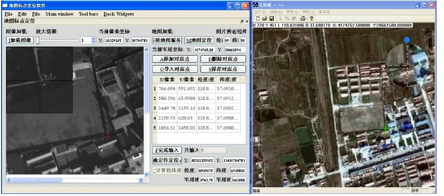
In order to test the algorithm, we made some codes on Qt platform. Figure 2 demonstrates the appearance of target location program. The left window shows the aerial image, and the right window shows a digital map integrated with DEM data. The pixel marked by a red cross is the target in the aerial image, and its corresponding point in the map is calculated, marked by a green cross. So the geographical position is naturally obtained, displayed on the panel.
SNR =40dB Mapping
models Xl/m Yl/m Zl/m Xl/m Yl/m Zl/m Xl /m Yl /m Zl /m
1 -35.831 -35.749 479.35 0.1856 0.1842 0.0837 0.86 0.971 0.65
2 -36.733 -36.526 476.80 1.7834e-3 1.7819e-3 2.9283e-3 0.013 0.194 3.2
3 -36.508 -36.491 477.07 1.7788e-3 1.7734e-3 3.1837e-3 0.212 0.229 2.93
4 -38.048 -37.909 - 0.0135e-3 0.0136e-3 - 1.549 0.317
-SNR =20dB
l
X /m Yl/m Zl/m Xl/m Yl/m Zl/m Xl /m Yl /m Zl /m
1 -37.008 -36.357 502.37 1.7987e-3 1.7857e-3 2.7765e-3 0.288 0.363 30.37
2 -36.219 -36.329 504.98 0.1852 0.1858 0.1689 0.501 0.391 24.98
3 -38.485 -36.927 499.24 0.1762 0.1777 0.3455 1.765 0.207 19.24
4 -37.58 -36.852 - 1.2096e-3 1.2805e-3 - 0.86 0.132
Figure 2. The appearance of location program.
5. CONCLUSIONS
This paper presents a pipeline of target location, in which the mapping model fits the transformation of correspondences, respectively from the aerial image and digital map. According to the diversity of unknown parameters, three forms of mapping models are discussed in detail, which could be suitable for different types of terrains. The associated error analysis is also elaborated, involving the location error of transferred target point. From the results of synthetic experiments, the positioning error is considerably small. Hence, this target-location strategy based on rich and high-precision data of digital maps is effective and economical for low-cost UAVs, even not equipped with high-performance platforms and POS.
REFERENCES
DongGyu, S., 2002. Localization based on DEM matching using multiple aerial image pairs. IEEE Trans. Image Process, 22(1), pp. 52-55.
G.N. Newsam, 1996. Recovering unknown focal lengths in self-calibration: An essentially linear algorithm and degenerate configurations. In: Int. Arch. Pho-togrammetry & Remote
Sensing, Vienna, vol. XXXI-B3, pp. 575-580.
Hongjian, Y., 1998. Error analysis and accuracy estimation of airborne remote sensing with air-to-ground positioning system.
Acta Geodaetica et Cartographica Sinica, 27(1), pp. 1-9.
Richard, H., 1997a. In defense of the eight-point algorithm.
IEEE Transactions on Pattern Analysis and Machine
Intelligence, 19 (6), pp. 580-593
Richard, H., 2003. Multiple View Geometry in Computer
Vision. Cambridge University Press, Cambridge, pp. 87-194.
Shaoli, X., 2005. Error analysis and accuracy estimation of air-to-ground positioning system based on GPS/INS. Bulletin of
Surveying and Mapping, 2005 (4), pp. 30-32.