A frost assessment method for mountainous areas
L. Lindkvist
a,∗, T. Gustavsson
a, J. Bogren
baForestry Board, West Sweden, Box 343, SE-503 11 Borås, Sweden
bGöteborg University, Department of Earth Sciences, Physical Geography, Laboratory of Climatology,
Guldhedsgatan 5C, SE-413 81 Göteborg, Sweden
Received 15 October 1997; received in revised form 26 July 1999; accepted 3 August 1999
Abstract
The present paper describes a model for frost assessment in mountainous areas in relation to forest management. Data were collected at 38 locations within a 625 km2region, which is characterised by a diverse topography and vegetation cover.
Air temperature measurements were performed during the peak of the growing season. (July–August 1996) in the southern Swedish mountains at elevations between 500 and 1200 m a.s.l. The variation in nighttime minimum temperatures was analysed in relation to the prevailing weather and terrain type of the measuring sites.
From the analysis of the temperature and weather conditions, i.e., wind and radiation, it was concluded that more than 90% of the frost situations, occurring during the study period, were of the radiation type. It was further concluded that the variation among the studied stations was closely related to the terrain type during these situations. Frost occurred most frequently in narrow valleys, then in concave and flat locations. Elevated and convex areas were found to have very few situations of radiation frost.
Local terrain information was used together with a calculated frost index for assessment of the spatial variation in frost risk. Furthermore, a grid net was applied to the study area and the pixels were given a terrain form of the type convex, slope, flat, wide concave or narrow concave according to the dominating terrain curvature. For each pixel a frost index value was estimated from the recorded temperatures at the field stations. A cluster analysis was used to group the terrain types according to the index, whereby six obvious clusters were obtained each with clearly differentiated frost intensity. The analysis showed that this kind of treatment is a suitable method for assessing the spatial variation in frost risk. © 2000 Elsevier Science B.V. All rights reserved.
Keywords: Growing season; Radiation frost; High elevation; Topoclimatology; Cluster analysis; Frost risk assessment
1. Introduction
Assessment of the local climate variability is an im-portant issue in sound forest management. It is a partic-ularly relevant component in areas with elevated boreal
∗Corresponding author. Tel.:+46-33-177331; fax:+46-33-177389.
E-mail address: [email protected] (L. Lindkvist)
forests, due to its exposed environment near the limit of physical tolerance for tree vegetation. Thus, moun-tain forests represent a thermally marginal ecosystem which is believed to show an early response to varia-tions in climate (e.g., Schlesinger and Mitchell, 1989; Mitchell et al., 1990).
The variability of low summer night temperatures is of crucial concern for the survival and progress of young trees as shown, for example, by Christersson
(1971) and Burke et al. (1976) and the implications of frost during the peak of the growing season is of specific importance for the establishment and devel-opment of conifer saplings (Li and Sakai, 1981; Sakai and Larcher, 1987). It should also be mentioned that the risk of injury might be high during the spring when buds are flushing and the apical shoots develop.
Furthermore, survival and yield of coniferous veg-etation is related in a broad sense to variations in altitude (Persson and Ståhl (1990). In this context, local terrain complexity plays an important role, i.e., marked variations in the topography leading to terrain constrictions with implications on the establishment of frost. Therefore, methods that point out hazardous areas with regards to clear-felling and succeeding plant regeneration are useful planning tools in the lo-cal management of elevated forests. Furthermore, it is important that such methods are general in their appli-cability and yet accurate in their usage across different areas, due to the strong variations in local climate that can be expected between different terrain types.
Information on the temperature distribution in different terrain, different latitudes and different el-evation is commonly used in indices and for classi-fications related to, vegetation distribution and tree growth, (e.g., Thornthwaite, 1931; Thompson, 1969; Ahti, 1970). Several authors have concerned them-selves with mapping of the bioclimate in Scandinavia (the temperature climate in particular), as it is related to the distribution of various types of forest ecosys-tems on both a regional and national scale (e.g., Ahti et al., 1968; Hustich, 1979; Tuhkanen, 1980; Odin et al., 1983). Often, such studies make use of variables which are closely related to temperature e.g., coldness sum, frost sum, heat sum, degree-days (d.d.), growth units and length of growing season. However, stud-ies on the temperature climate or related expressions that are applicable to a local mountainous terrain are less frequent. There are several obvious reasons to this, for example, the network of synoptical meteo-rological stations becomes less dense in mountainous regions and consequently does not support local cli-mate applications. Also, the mountainous areas are often vast, have low accessibility and are, therefore, more difficult to assess manually.
Early works concerning frost investigations dealt primarily with empirical formulae for specific areas such as orchards, where anticipated low temperatures
and the duration of temperatures at certain levels are predicted. The frost risk is often calculated from an analysis of the energy balance and heat transfer pro-cesses near the surface. Several of the empirical mod-els are derived from the Brunt equation (Brunt, 1944). Several authors have performed mapping of tem-perature variations and variation in local frost risk. Lomas et al. (1989) have analysed a large number of temperature recordings in order to produce local-frost risk maps. These maps show the number of occasions expected for selected sub-regions in relation to long term data. More sophisticated models have also been developed such as the three-dimensional local scale numerical models for simulation of the microclimate near the ground surface in complex terrain (Avissar and Mahrer, 1988).
The present project is focused upon the establish-ment of minimum temperature variation during differ-ent weather situations in relation to terrain types. The purpose is to develop a method for a terrain division that accounts for a high proportion of the local vari-ability of summer frost in elevated, complex terrain. Such an empirical model could further be used for other areas, i.e. the method should be based on general parameters which could be determined for new areas with little or no help from measurements.
2. Characteristics of the study area
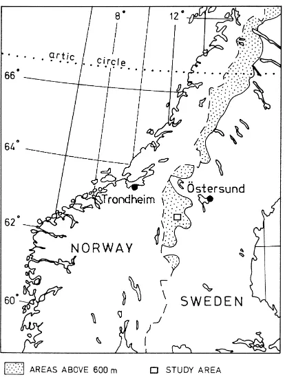
Fig. 1. The location of the study area in the southern part (62–64◦N) of the Scandinavian mountain range (Scandes). The location of areas above 600 m a.s.l. in the Scandes are included for the Swedish side.
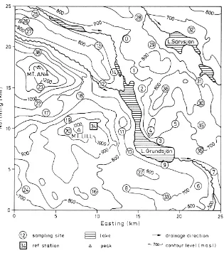
500 and 1400 m a.s.l. A detailed map of the study area showing relief contours, lakes and mountain peaks is provided in Fig. 2.
The weather of the study area can be characterised as an alternation of low pressure systems frequenting the region most frequently from the west and periods (2–5 days) in between with anticyclone conditions. Periods of blocking highs are also relatively frequent. During such longer clear periods frosts are experi-enced. This has important implications for plant injury and mortality of conifers during the peak of the grow-ing season (July–August) and in sprgrow-ing at the time when flushing and the development of apical shoots takes place.
During the most recent standard period, 1961–1990 (SMHI, 1991) the nearby synoptic weather station at Fjällnäs, located 30 km west of the study area at 780 m showed an annual average temperature of
−0.4◦C. The mean temperatures for July and August
are 10.5 and 9.4◦C, respectively. At mean height of the study area (750 m) the annual average tempera-ture was−0.2◦C and the monthly averages for July and August were 10.9 and 9.5◦C, respectively, for the period 1994–1996.
The growing season normally starts at the beginning of June and extends to mid-September. Based on the measuring period 1961 to 1976 the average length of the growing season for the region has been established by Odin et al., (1983) to 120–140 days and the tem-perature sum to 550–650 d.d., threshold value+5◦C).
These numbers are reduced to less than 110 days and 530 d.d. at mean height in the study area.
Mountain birch (Betula pubescens subspecies (ssp.)
tortuosa) forms the tree-line at approximate elevations
between 850 and 1000 m above sea-level and are gen-erally frequent above 800 m. However, in the south-ern part of the region, conifers occasionally form the tree-line without the presence of any birch. At heights between 750 and 800 m, poorly developed and widely spaced conifers (Picea abies ssp. and Pinus silvestris) usually dominate the forests. Birch intermingles to a various degree with pine and spruce in this zone of transition.
The distribution of trees is obviously associated with altitude. The coniferous vegetation tends to show a gradual improvement in progress as height above sea-level decreases, however the complexity of the ter-rain has a strong influence on the distribution. Thus, in local areas like valleys and low level terrain down to 600 m, trees may be completely absent, i.e. inverted tree-line, or show a highly reduced development. In-clined ground, particularly south and southwest facing slopes exhibit the best environments for tree growth in the study area.
Fig. 2. Topographical map over the study area, the temperature sampling locations are shown.
3. Methods and materials
3.1. Acquisition of climate data
Temperature data was sampled at 38 locations for 60 consecutive days during the growing season of 1996. The sampling sites were distributed over a 625 km2 area of highly complex terrain shown in Fig. 2. The altitude and terrain form associated with each sam-pling location is presented in Table 2. The locations comprise a variety of local climate environments, all in open or clear-felled terrain with low vegetation of grass, twigs and plants. The purpose of this sam-pling scheme was to spatially partition the temperature
distributions that evolve in different terrain types in a region with strong relative relief.
diameter 10 cm) are then orientated in a north–south direction, cut obliquely at the ends and tilted 40◦ to the horizontal in order to prevent direct sunlight and stagnation of air from influencing the measurements.
A reference station measuring temperature, wind speed, wind direction and net radiation was estab-lished at 1020 m on Mt. Lill (Fig. 2). The measuring equipment consisted of temperature sensors (Platinum 100, accuracy 0.1◦C), a cup anemometer (threshold value 1.0 m s−1), a wind vane (Young Wind Monitor,
R.M. Young Co., Traverse City, MI, USA) and a net radiometer (Q-7, Radiation Energy Balance Systems, Seattle, WA) with wind effect less than 1% for neg-ative fluxes up to 7 m s−1. Data were recorded every 10 min and hourly averages were stored on a Camp-bell data-logger (CampCamp-bell Scientific, Logan, UT).
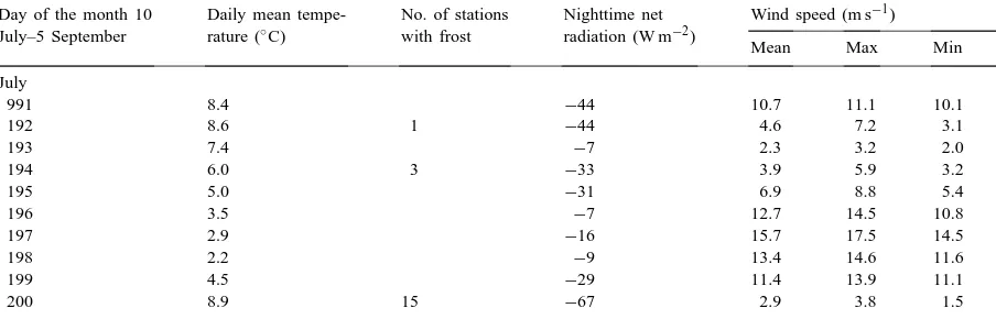
The measurement period encompassed a wide range of different weather conditions (see Table 1). From the data it was possible to categorise the weather de-pending on the prevailing cloudiness and wind. The nighttime net radiation was used as criteria for differ-entiating between clear and cloudy weather conditions as minimum temperature and frost occurrence formed the main focus of this study. During the night, the net radiation equals the long wave radiation incom-ing from the sky minus the outgoincom-ing long wave radi-ation from the ground. The incoming part is mainly a function of air temperature, humidity and cloud cover, with cloud cover dominating. Thus, the variability observed between different nights is mainly a result of variable cloud cover. According to calculations made
Table 1
The weather (daily mean temperature and wind speed, frost occasions and nighttime net radiation) during the measuring period from 10 July to 5 September 1996
Day of the month 10 Daily mean tempe- No. of stations Nighttime net Wind speed (m s−1)
July–5 September rature (◦C) with frost radiation (W m−2)
Mean Max Min
by Perttu (1981) of net long wave radiation for clear nights (based on the formulae by Ångström, (1974) and Brunt (1944) typical values of −65 W m−2 or lower were obtained
In this study the weather is categorised as clear if the net radiation is below−40 W m−2and cloudy if the net radiation is above−20 W m−2. The 60-day measuring period comprises 27 nights that are classified as clear while 16 are categorised as cloudy, with the others being intermediate; i.e. a good coverage of different types of weather conditions was obtained during the measurement period. During the investigated period frost occurred at 26 occasions, i.e., at least one of the stations in the area had temperatures below 0◦C.
3.2. Terrain forms – site description
A ground based satellite aided navigation equip-ment (GPS), which provides position fixes to within 30 m (Silva XL 1000, SILVA Sweden AB) was used in order to spatially define the locations of temperature sampling sites and the reference station.
Table 1 (Continued)
Day of the month 10 Daily mean tempe- No. of stations Nighttime net Wind speed (m s−1)
July–5 September rature (◦C) with frost radiation (W m−2)
Mean Max Min
201 10.4 11 −66 3.2 5.0 1.5
202 10.8 −30 5.3 6.0 4.5
203 11.4 −33 3.6 4.8 2.2
204 12.3 −23 4.2 5.6 2.3
205 12.0 −30 6.1 6.7 4.2
206 9.2 −29 4.4 5.6 3.5
207 7.4 13 −68 3.8 6.5 1.2
208 7.6 −2 7.1 8.6 5.4
209 5.9 −31 4.4 8.0 0.5
210 3.8 −42 7.9 11.1 5.8
211 4.3 −43 10.6 12.3 9.4
212 6.7 12 −44 3.5 5.4 1.5
August
213 7.6 7 −5 9.2 10.6 8.3
214 5.6 −5 9.2 10.6 8.3
215 4.6 −7 12.0 13.9 10.3
216 6.7 −17 7.8 8.2 6.5
217 10.6 −20 3.4 5.8 1.5
218 13.0 2 −65 5.4 5.7 5.0
219 12.3 2 −66 6.6 7.6 5.9
220 11.3 3 −55 5.7 6.5 4.8
221 10.4 −24 7.7 8.7 6.9
222 10.4 −38 8.3 9.0 6.9
223 11.8 4 −71 8.3 9.0 7.3
224 12.9 −57 6.1 7.0 5.2
225 13.0 3 −68 6.8 7.7 6.0
226 13.3 1 −68 7.4 8.3 6.7
227 12.2 3 −62 5.5 7.2 3.2
228 12.4 −40 3.2 4.3 2.7
229 11.6 −34 6.7 7.4 5.8
230 10.7 2 −29 2.2 4.2 0.6
231 13.5 −46 8.5 10.4 7.5
232 14.5 1 −66 8.1 10.4 6.6
233 14.5 1 −66 6.9 8.6 5.5
234 11.9 −53 3.6 4.2 3.3
235 10.4 −2 5.1 5.9 4.1
236 11.1 −4 5.6 6.3 4.5
237 10.5 −1 9.6 11.5 7.0
238 9.8 −2 5.9 7.2 4.9
239 9.0 −3 4.7 6.9 2.7
240 9.3 −3 7.4 8.5 6.4
241 10.1 5 −64 4.8 6.5 3.0
242 9.4 −1 7.2 8.5 5.7
243 7.4 1 −28 5.5 7.3 2.4
September
244 7.0 −11 9.5 10.9 7.8
245 9.1 2 −46 9.1 10.5 6.5
246 6.8 −60 8.7 11.2 7.2
247 2.1 −32 12.8 14.8 9.9
along several topographical cross-sections in IDRISI, a GIS software developed by Eastman (1992). The ter-rain categories that were defined in this way include five principal types: (1) convex terrain: ∩, (2) linear sloping terrain:↓, (3) linear flat:↔, (4) wide concave terrain:∪and (5) narrow concave terrain:∨. In Table 2 information regarding the altitude and type of terrain are included for each sampling location.
Convex terrain (peaks and ridges) are found mainly at elevations above 800 m. Four areas are identified in Fig. 2. Two broad peaks above 1100 m (Mts. Anå and Lill) , a ridge reaching 1000 m north of the peaks and a broad convex area east of the peaks at 800–950 m. Two types of valleys, narrow and wide concavities, are present in the same figure. The former varies in width between 1.0 and 2.0 km, whereas the latter is 2.5–4.0 km wide. The narrow type is located between Mt. Anå and Mt. Lill and the wider type follows the two rivers and surrounds L. Grundsjön and L. Särvsjön.
The areas surrounding L. Grundsjön are considered flat, i.e. less than 3◦inclination. A 5–7 km wide level area divides the concavities in the northern part of the study area. Open level ground is also identified in the southeast corner of Fig. 2. Thus, this terrain type vir-tually bisects the study area from north to southeast, leaving valleys and hilltops at each side. The remain-ing terrain type, i.e. slopes (more than 3◦inclination), connects the convex hilltops and ridges with concav-ities and flat valley floors. Differences in slope incli-nation are not considered due to the fact that sloping terrain is known to show only small variations in frost susceptibility compared to the variations that occur across different terrain types defined in this study.
Table 2
Altitude and dominating terrain form at 38 sampling locations. Each location is assigned one of the five major terrain forms that were defined according to its curvature; convex, concave, linear sloping and linear flat. The symbols are included in order to simplify the comparison between tables and figuresa
Sampling site 0 1 2 3 4 5 6 7 8 9 10 11 12 13 14 15 16 17 18
Altitude (m a.s.l.) 710 700 670 680 870 680 630 600 710 670 680 710 670 720 660 710 830 780 740
Terrain form ↔ ↓ ↔ ↓ ∩ ↓ ↔ ↔ ↓ ↓ ↓ ↔ ∨ ↓ ↔ ↓ ↔ ∨ ∨
Sampling site 19 20 22 23 24 25 26 27 28 29 30 31 32 33 34 35 36 37 38
Altitude (m a.s.l.) 950 1120 950 1110 680 710 830 995 680 700 790 650 660 700 1080 680 880 780 940
Terrain form ↓ ∩ ↓ ∩ ↓ ∨ ∩ ∩ ∪ ↔ ∩ ↓ ∪ ↓ ∩ ↓ ∩ ∩ ↓
a↔: flat area, surface inclined<3◦;↓: slope, surface inclined >3◦;∩: convex area;∪: wide concave area (U-shaped valley); V=narrow concave area (V-shaped valley).
4. Results and discussion
4.1. The influence of elevation and local terrain on the establishment of low temperatures
Investigations have shown that local topography may cause large temperature variations to develop e.g., Marth (1986); Toritani (1990); Bogren and Gus-tavsson (1991). Several studies have been concerned with investigations of temperature variations at low points in the terrain, e.g. Catchpole (1963); Dight (1967); Doran and Horst (1983); Miller et al. (1983). A division based on weather conditions is necessary in order to assess the role of different topographical parameters. The following discussion is based on the variation expected during the two most extreme situ-ations; cloudy, windy nights and clear calm nights. In order to benefit from frost risk models it is necessary that different weather types are treated accordingly.
During cloudy, windy conditions the counter-radiation and high percentage of diffuse counter-radiation will lead to a smoothing of local temperature variation. Furthermore, the wind itself will aid in this process by increasing turbulence. The temperature stratifica-tion can be described as neutral or unstable, i.e. a temperature decrease with increasing height above the ground. For frost risk studies, this weather type is of major significance as advective frost can occur during these situations.
Fig. 3. Relationship between the differences in minimum temperature at different locations and that at the reference site and altitude above sea level of the measurement location during cloudy and windy conditions. y= −0.0062x+6.74, R2=0.925.
wind speed exceeding 6 m s−1 have been attained. The averages of these differences versus altitude have been plotted for each logger location, Fig. 3. There is a very good correlation (R2=0.93) This implies that the general decrease in temperature during this type of weather controls the differences between the sta-tions. The lowest nighttime temperatures are found at the highest altitudes and the warmest temperatures are located in the lowest areas. This relationship accords well with the physical processes described above and has been shown to be valid in several studies, e.g. Kalma et al. (1986).
During clear, calm nights the variation in mini-mum temperature is to a large extent controlled by the possibility of cold air accumulation. Cold air accumulates at low points such as valley bottoms due to the fact that cold air is denser than warm air. Other factors, which have been shown to be of great importance, are the degree of shelter. In a sheltered location the mixing of surface cold air with warmer air aloft is reduced. The effect resulting from this has been demonstrated in studies by e.g. Tabony (1985); Gustavsson (1995); Gustavsson et al. (1998). Shelter can be both in the form of topography, e.g. narrow valleys, small hills, or in the form of vegetation, i.e. tree stands or lines of trees.
The variation in minimum temperature for clear nights (radiation<−0 W m−2; wind speed<8 m s−1) has been analysed in a similar way as for the cloudy,
windy situations described above. In Fig. 4, the av-erage difference in minimum temperature versus the reference station has been plotted against altitude of the site. As can been seen in the figure the scatter be-tween the stations is large. A trend can be seen that the low-lying stations are in general colder than the higher sited ones. However, the temperature values clearly show that a linear correlation would only describe a small part of the variation, R2=0.40 for the linear fit with Y=0.0147X–14.87.
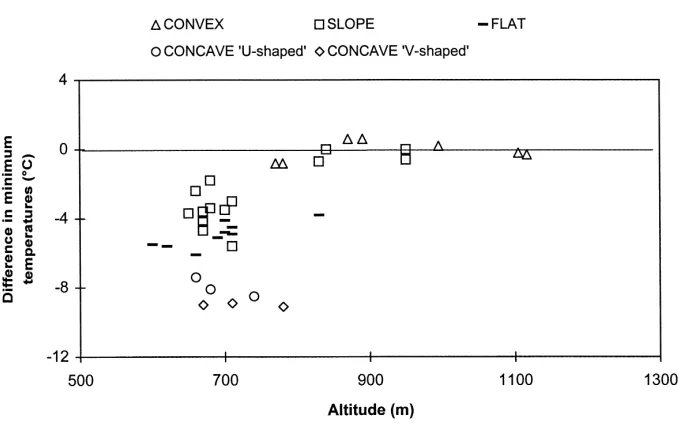
In Fig. 4 the local topography for each site has been included following Table 2. However, the concave ar-eas have been treated as one. It is clear from this figure that the local topography has a much larger influence on the temperature difference than the height above sea level.
Fig. 4. Relationship between the differences in minimum temperature at different locations and that at the reference site and altitude above sea level of the measurement location during clear and calm weather conditions.
the station is of greater importance compared with elevation.
To further study the influence of local topography on the variation in minimum temperature during clear nights the data from Fig. 4 have been used. The mean variation has been calculated for each type of location as described above (see Table 2). To be able to com-pare the data presented in this study with the figures
Fig. 5. Comparison between two temperature sampling locations at the same height above sea level but in different terrain. Station 17 is sited in a narrow concave valley. Station 37 is located on a ridge (see Fig. 2)
presented in the studies by Kalma et al. and Laugh-lin and Kalma, the same elevation interval has been included in the table, i.e. 160 m.
argued that a frost assessment model in complex ter-rain should not just be based on altitude for prediction of minimum temperature during clear nights. In the above-cited studies the residuals were used to describe the influence from topography, especially drainage of cold air to valleys. However, for the type of topogra-phy classified in this study, this kind of method ex-plains only a smaller part of the variation. This is due to the fact that the scatter among the linear fit is too large and that the residuals can amount to nearly 6◦C,
i.e. more than half of the total variation in nighttime minimum temperature versus the reference station.
The reason why a good correlation was obtained be-tween minimum temperature and elevation in several previous studies is probably due to the fact that only one major valley system has been studied. If one plots the temperature variation for a single profile including the terrain types, convex, slope and concave, a good correlation is achieved. However, if a more complex system is studied then different types may be found at different altitudinal levels and thereby the correlation between elevation and temperature variation is nulli-fied. These findings are in agreement with previous studies that have shown that there is a low correlation between elevation and minimum temperature during clear, calm nights, e.g. Avissar and Mahrer (1988), Gustavsson (1995).
Another important aspect regarding the modelling of temperature variations is the ability to handle the
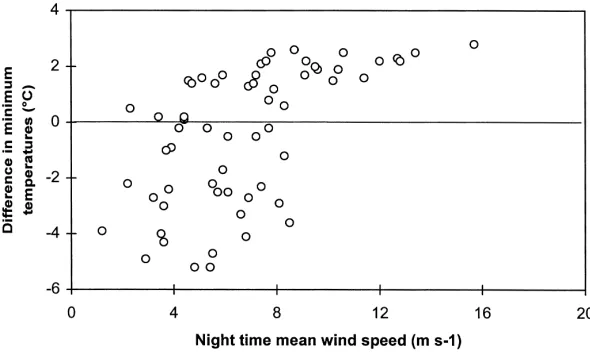
Fig. 6. Differences in minimum temperature at different wind speeds calculated for Station 17 and the reference station (1020 m).
large number of weather situations that occur between the two extremes already discussed. Several studies have focused upon the task of determining the rela-tionships between wind speed and amount of cloud with net radiation. In studies by Gustavsson (1990) and Bogren and Gustavsson (1991), the importance of the prevailing wind speed and cloud cover for the de-velopment of large temperature differences has been discussed. Others e.g., Bootsma (1976) and Laughlin (1982) have related temperature differences in com-plex terrain to both radiation and wind speed by em-pirical formulae. The influence from cloud ought to be the same between different areas as it basically con-trols the amount of outgoing long-wave radiation. The influence from the prevailing wind speed, on the other hand, is more likely to show a large variation from place to place owing to such factors as topography and local wind shelters.
In Fig. 6 the temperature differences for all 60 nights with varying wind speed have been plotted. A very sharp difference can be seen for nights with mean nighttime wind speeds exceeding 8 m s−1 and nights with those below. Comparison for other stations in the area gives similar results. The reason for such high limits (8 m s−1) and the fact that below that limit the
effect which significantly reduces the turbulent mix-ing between the surface cooled air and warmer aloft. The data in Fig. 6 clearly demonstrates the importance of wind shelter as a major factor for the development of large temperature differences.
4.2. Frost under different weather conditions
In the previous section it was shown that the local topography together with altitude acts as a controlling factor for temperature variation. Normally two types of frost situation can be distinguished, radiation and advective frost. Advection frost occurs during situa-tions where cold air intrudes into an area. This results in the lowest temperatures at the elevated sites, i.e. a temperature decrease with height as already discussed. Radiation frost on the other hand, occurs during situa-tions with in-situ cooling, i.e. clear sky and low wind speed. The temperature, wind speed and net radiation for the study period is presented in Table 1 along with the number of stations with frost situations at night-time. All frost situations that occurred during this time period can be classified as radiation frost.
One way of estimating the local frost risk for a spe-cific location is by adding the number of situations with temperatures below 0◦C. Calculations of frost
sum and coldness sum (day-degrees) below a certain threshold value are commonly used methods for quan-tifying the frost risk at different areas (cf. Tuhkanen, 1980). However, such indices are general in their char-acter in that they do not refer to any specific type of risk.
Lindkvist and Chen (1999) introduced a more comprehensive index. Their summation is based on occasions with temperatures below 0. Furthermore, each situation was subdivided with relation to local conditions such as the time period of freezing temper-atures as well as a division into temperature levels. The temperature level division is used to take into account how much the temperature will fall below 0. Furthermore, a weight factor is applied to each of the levels according to the increasing risk of plant injury given that, successively colder situations are more im-portant to consider. The index was found to account for more than 80% of the variability in mortality, mea-sured 5 years after re-planting in the above mentioned study. Therefore, the index composes a measure of frost intensity and provides an indication of the risk
of plant re-growth failure in different types of terrain. In order to analyse the relation between the local topography and local frost risk, the Lindkvist–Chen index was calculated for radiation frost situations and presented together with topographical information in Table 4. The table combines information concerning altitude and terrain form at the different sampling lo-cations. The number of frosts and the calculated index were also included. The table was sorted according to increasing index values. The relationship between terrain curvature and low summer night temperatures becomes obvious in this arrangement.
4.3. Terrain classification and temperature estimation
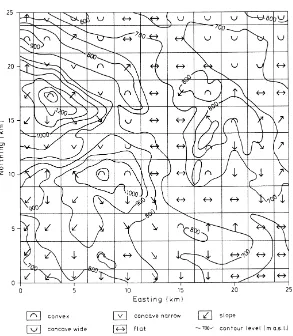
To be able to estimate the spatial variation in frost risk of radiation Type A grid was applied to the study area and the pixels were classified according to the ter-rain curvature. The symbols used for different curva-ture are superimposed on a terrain map and presented in Fig. 7. The grid pixels cover an area of 2.5/2.5 km except for those along the borderline of the study area, which are half in size. Consequently, the choice of terrain curvature that defines a pixel follows the dom-inating type.
Index values (Lindkvist–Chen index) were calcu-lated for each one of the 38 measuring stations. It was then possible to group a specific index value, or a range of values, with a defined terrain form for pixels with temperature observations. In order to ex-tend this procedure to cover all the pixels in the study area 121 index values where estimated by applying a geostatistical method to the data-set containing the calculated index. The method (kriging) uses a local weighted moving average technique that offers a way in which to minimise the variance of the estimation error. This technique is thoroughly described in sev-eral textbooks (e.g., Issacs and Srivastava, 1989 and Englund and Sparks, 1988). Furthermore, applications similar to the one used in the present study are avail-able in Söderström and Magnusson, (1995) and Lind-kvist and Lindqvist (1997).
Fig. 7. A classification of terrain elements in the study area. Single arrows indicate the major drainage direction on slopes. (1)∩ =convex. (2)↓ =slope. (3)↔ =flat. (4)∪ =wide concave (U-shaped valley). (5)∨ =narrow concave terrain (V-shaped valley).
kriging standard deviations, therefore it was decided to exclude estimates showing kriging SD higher than 10.
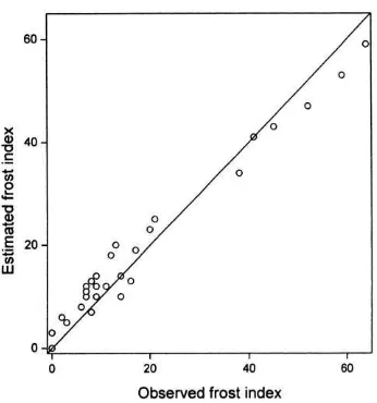
To verify the results from the Kriging procedure, where an average of three to four estimates were pro-duced for each observed value, a cross-validation was carried out between the 38 calculated index values based on temperature observations and 38 index val-ues based on estimations at the same locations. Fig. 8 gives the results of the difference between observed and estimated values. A very high correlation coeffi-cient (0.97) was achieved, which indicates a low level of estimation error in the interpolation.
Since more extreme observations will show a greater difference to the estimated values in the interpolation a 1 : 1 line was included in the
fig-ure to explain the degree of smoothing. A slight over-estimation occurs for values in the lower range of the index and under-estimation is present in the upper range. However, the deviations are generally very small. Since there is an abundance of stations showing over-estimation, a small increase in the index average from 17 to 19 is noted.
Fig. 8. Comparison of estimated against observed frost index values. R2=0.98.
transitions can be seen in Table 3, e.g., the calculated index leaps from 26 to 52 when concave terrain is encountered. A stepwise increase can be explained by the fact that sampling of intermediate terrain forms is avoided in order to isolate the main types in this study. A lower slope that is entering gradually a concave curvature is an example on intermediate terrain form. It is evident from Table 3 that different terrain types can be connected to specific ranges of frost intensity. If such a relationship is highly significant it can allow a simplification of frost risk assessment. In order to investigate the possibility of applying the established relation in the entire study area, the estimated index was subject to cluster analysis.
Different methods for cluster analysis exist, how-ever they are all designed to minimise the within-group deviation of the observed variable and to maximise the between-group deviation. Euclidean distance (in this case, a summation of the difference squared between frost index values separated by a known distance) was
Table 3
Calculated mean difference in minimum temperature versus the reference station for four types of topographical locations.
Site Convex Slope Flat Concave
Altitude interval 160 m −0.8 −3.6 −5.0 −8.4 Altitude interval 520 m −0.1 −2.7 −4.9 −8.5
used to calculate the dissimilarity between the esti-mated index values. The clusters were obtained ac-cording to Ward’s method, see for example Burrough (1986).
In the analysis each index value was given a terrain ‘signature’ according to the five terrain categories defined. Three main clusters (A–C) are prominent (Table 5). Also, two sub-groups in each cluster (low and high) are apparent. The terrain categories are identified at the sub-group level. By the cluster anal-ysis it is inferred that different types of flat areas should be treated separately depending on their loca-tion relative to the surrounding terrain. Furthermore, convex terrain together with exposed and elevated slopes should obviously form a common group while lower and shaded slopes should compose a separate entity. Wide and narrow concavities remain as pre-vious in two unique groups. However, as discussed by previous authors, e.g. DeGaeteno and Schulman (1990), there is no definite method to decide on for an optimum number of clusters and/or sub-clusters. Thus, it is to a certain degree an arbitrary choice.
It was assumed that three to five groups of distinct terrain forms with possible sub-divisions would be an appropriate number in order to distinguish between areas of different frost risk. As an objective selection method for the introduction of new clusters, a simple technique of looking at mean values and standard de-viations (SD) was applied to find out the final number of clusters to be considered.
Table 4 lists the mean, range and standard deviation of the clusters that were examined. The terrain classes are included in the table to compare between ranges of index values and type of terrain. Clusters B and C show the two most evident sub-groups, which are accompanied by a distinct lowering of the SD. For Cluster A, the SD is already low, however a further reduction motivates a division. Terrain categories and clusters are matched in the table and three main groups and two sub-levels in each group are formed, each with a unique frost risk.
4.4. Frost risk evaluation
Table 4
The relationship between altitude, terrain form, number of frost occasions and frost index values for 38 sampling locations in the study area. The index values are compiled with the method presented by Lindkvist and Chen (1999)
Site Altitude (m a.s.l.) No. of frosts Index value Convex∩ Slope↓ Flat↔ Concave wide∪ Concave narrow∨
4 870 0 0 ∩
30 790 0 0 ∩
36 880 0 0 ∩
37 780 0 0 ∩
26 830 0 0 ∩
27 995 0 0 ∩
34 1080 0 0 ∩
23 1110 0 0 ∩
20 1120 0 0 ∩
38 940 0 0 ↓
22 950 0 0 ↓
19 950 0 0 ↓
24 680 2 2 ↓
9 670 2 3 ↓
8 710 2 6 ↓
31 650 2 7 ↓
10 680 3 7 ↓
1 700 3 7 ↓
35 680 3 8 ↓
15 710 4 8 ↓
3 680 4 9 ↓
5 680 4 9 ↓
33 700 4 9 ↓
16 830 6 11 ↔
0 710 4 12 ↔
13 720 4 13 ↓
6 630 5 14 ↔
2 670 4 14 ↔
11 710 4 16 ↔
7 600 5 17 ↔
14 660 5 20 ↔
29 700 5 22 ↔
28 680 10 37 ∪
18 740 11 39 ∨
32 660 13 45 ∪
25 710 16 50 ∨
12 670 18 58 ∨
17 780 19 62 ∨
grid net of terrain categories Fig. 7) a specific cluster of the estimated frost index according to the relation-ship shown in Table 5. Thereafter, the borderlines of clusters that are members of the same sub-group are delineated. Thus, the map in Fig. 9 show six different patterns equivalent to six levels of frost risk. Three unique patterns are used, one for each of the main frost risk levels. By differentiating the intensity of each pat-tern, it is possible to distinguish between main groups and sub-groups according to the legend in the figure.
Note that areas above 850 m are excluded due to the fact that forestry is not normally practised above this height in Sweden.
Fig. 9. Map over the study area showing 6 levels of frost risk. (1) very low, (2) low, (3) intermediate, (4) high, (5) very high and (6) extreme risk.
Table 5
Results of cluster analysis on frost index values and basic statistics for the different clusters. The main cluster levels are marked A–C. Low and high marks the sub-cluster
Main clusters and subtypes Index mean Index range SD Terrain class Frost Risk evaluation
A 9 2–12 3.0 ∩,↓ low
Low 4 2–7 2.0 ∩,↓
High 10 9–12 1.0 ↓
B 24 16–35 6.4 ↔ intermediate
Low 19 16–22 2.0 ↔
High 31 28–35 2.7 ↔
C 49 39–64 7.2 ∪,∨ high
Low 43 39–48 3.0 ∪
the high-risk level are highly related to the surround-ing terrain, i.e. areas located adjacent to cold valleys that open up into wider terrain and in the transition from wide concavities to flat areas.
The second highest risk level (very high) is syn-onymous with broad concave areas, which are mainly a part of large ‘U-shaped’ valley bottoms. Beside in situ production of cold air, accumulation from the sur-rounding slopes and plateaux account for the high level of frost risk in these areas. Narrow ‘V-shaped’ con-cavities are found to be extremely frost prone due to the high degree of wind shelter and accumulation of cold air.
5. Conclusions
Radiation frost was found to be the dominating type of frost during the peak of the growing season. Radi-ation frost is strongly favoured by the high degree of wind shelter and shade that a terrain of pronounced concave–convex complexity offers. Thus, terrain cur-vature is found to be an important variable that must be taken into account when assessing the summer frost risk in mountainous complex terrain.
A strong relationship between frost intensity and terrain form was established in this study. This mo-tivates the use of a simplified method for assessment of frost risk in complex terrain. In order to carry out such an assessment the following steps should be con-sidered: (1) a grid net should be superimposed with a map of the study area containing elevation contours to facilitate a classification of terrain forms. (2) One of six major types of terrain forms need to be identified in each pixel; concave areas (two types available), flat
ar-eas (two types available), sheltered/shaded slopes and exposed slopes/convex areas, (3) field control and/or
comparison with aerial photographs for verification of the terrain classification. (4) Delineation of units con-taining similar terrain forms and a ranking of frost risk levels.
6. Recommendations
Due to the empirical nature of the method, it is desirable that some kind of calibration factor is ap-plied prior before its use in new areas. Therefore, it is
recommended that a limited number of observations are allocated to the type of terrain that corresponds to the major frost risk levels in the present study. Such a procedure would require a minimum of three obser-vations at carefully selected locations (hilltop, low flat ground and a basin area). In this way, a simple ver-ification of the approximate range of the frost inten-sity can be performed with little effort. Furthermore, it is recommended that the measurement period is ex-tended throughout the peak of the growing season, i.e. July and August or an equivalent period depending on the location of the investigated area.
Based on the results from the present investiga-tion and the results presented by Lindkvist and Chen (1999), recommendations are issued concerning the suitability for re-growth in elevated complex terrain. According to frost risk alone, areas defined by low or very low risk levels are considered suitable for forestry, however with consideration being given the elevated location of the area. Areas of intermediate risk are uncertain in this respect and high/very high levels are rated as unsuitable. Hence, highly unsuitable terrain is equivalent to areas showing extreme levels of frost risk.
References
Ahti, T., 1970. A map on the boreal subzones in eastern Canada. Dendrol. Seur. Tied. 1 (4), 2.
Ahti, T., Hämeth-Ahti, L., Jalas, J., 1968. Vegetation zones and their sections in northwestern Europe. Annals. Bot. Fenn 5, 1–28.
Avissar, R., Mahrer, Y., 1988. Mapping frost-sensitive areas with a three-dimensional local-scale numerical model Parts I and II, J. Appl. Meteor. 27.
Bogren, J., Gustavsson, T., 1991. Nocturnal air and road surface temperature variations in complex terrain. Int. Climatol. 11, 443–445.
Bootsma, A., 1976. Estimating minimum temperature and climatological freeze risk in hilly terrain. Agric. Meteorol. 16, 425–443.
Brunt, D., 1944. Physical and Dynamical Meteorology. University Press, Cambridge, 428 pp.
Burke, M.J., Gust, L.V., Quamme, H.A., Weiser, C.J., Li, P.H., 1976. Freezing and injury in plants. Annu. Rev. Plant Physiol. 27, 507–528.
Burrough, P.A., 1986. Principals of Geographical Information Systems for Land Resources Assessment. Oxford Scientific Publications, pp. 194.
Christersson, L., 1971. Frost damage resulting from ice crystal formation in seedlings of spruce and pine. Physiol. Plant. 25, 273–278.
DeGaeteno, A.T., Schulman, M.D., 1990. A climatic classification of plant hardiness in the United States and Canada. Agric. For. Met. 51, 333–351.
Dight, F.H., 1967. The diurnal range of temperature in Scottish glens. Met. Mag. 97, 327–334.
Doran, J., Horst, T.W., 1983. Observations and models of simple nocturnal slope flows. J. Atmospheric Sci. 40, 708–717. Eastman, J.R., 1992. IDRISI 4.1. Clark University. Graduate
School of Geography, Worcester, MA, USA, pp. 209. Englund, E., Sparks, A., 1988. Geostatistical Environment
Assessment Software – Users Guide: Environmental Monitoring Systems Laboratory, US Environ. Protection Agency, USA. Gustavsson, T., 1990. Variation in road surface temperature due
to topography and wind. Theor. Appl. Climatol. 41, 227–236. Gustavsson, T., 1995. A study of air and road surface temperature variations during clear windy nights. Int. J. Climatol. 15, 919– 932.
Gustavsson, T., Karlsson, M., Bogren, J., Lindqvist, S., 1998. Development of temperature patterns during nocturnal cooling. J. Appl. Meteorol. 37, 559–571.
Hustich, I., 1979. Ecological concepts and biographical zonation in the north: the need for a generally accepted terminology. Holarctic Ecol. 2, 208–217.
Issacs, E.H., Srivastava, M.R., 1989. An Introduction to Applied Geostatistics. Oxford University Press, pp. 561.
Kalma, J.D., Laughlin, G.P., Geen, A.A., O’Brien, M.T., 1986. Minimum temperature surveys based on near-surface temperature measurements and airborne thermal scanner data. J. Climatol. 6, 413–430.
Kalma, J.D., Laughlin, G.P., Caprio, J.M., Hamer, P.J.C., 1992. Advances in Bioclimatology 2 – The bioclimatology of frost, its occurence, impact and protection, 1-144. Springer Verlag, Berlin.
Laughlin, G.P., 1982. Minimum temperature and lapse rate in complex terrain: influencing factors and prediction. Arch. Meteorol. Geophys. Bioclimatol. 30, 140–152.
Laughlin, G.P., Kalma, J.D., 1987. Frost hazard assessment from local weather and terrain data. Agric. For. Meteorol. 40, 1–16. Laughlin, P., Kalma, J.D., 1990. Frost risk mapping for landscape planning: a methodology. Theor. Appl. Climatol. 42, 41–51. Li, P.H., Sakai, A., (Eds.) 1981. Plant cold hardiness and freezing
stress, Academic Press Inc. NY. 2 (3) 199–527.
Lindkvist, L., Chen, D., 1999. Air and soil frost indices in relation to plant mortality in elevated clear-felled terrain in Central Sweden. Climate Res. 12, 65–75.
Lindkvist, L., Lindqvist, S., 1997. Spatial and temporal variability of nocturnal summer frost in elevated complex terrain. Agric. For. Meteorol. 87, 139–153.
Lomas, J., Shashhoua, Y., Cohen, A., 1989. Mobile surveys in agrotopoclimatology. Meteorologische Rundschau 22, 96–101. Marth, L., 1986. Nocturnal topoclimatology. World Climate
Programme, World Meteorological Association, 1–76. Miller, D.R., Bergen, J.D., Neuroth, G., 1983. Cold air drainage
in a narrow forested valley. For. Sci. 29., 357–370.
Mitchell, J.F.B., Manabe, S., Tokioka, T., Meleshko, V., 1990. Equilibrium climate change. In: Houghton, J.T., Jenkins, G.T., Ephraums, J.J. (Eds.), Climate Change, The IPCC Scientific Assessment. Cambridge University Press, Cambridge. 131–172 Odin, H., Eriksson, B., Perttu, K., 1983. Temperature climate maps for Swedish forestry. SLU – Swedish University for Agricultural Sciences, Dept. For. Ecol. For. Soils, 451–57 (in Swedish with English abstract and figure text)
Persson, B., Ståhl, E.G., 1990. Survival and yield of Pinus sylvestris L. as related to provenance transfer and spacing at high altitudes in northern Sweden. Scand. J. For. Res. 5, 381– 394.
Perttu, K., 1981. Climatic zones regarding the cultivation of Picea abies L. in Sweden II. Radiation cooling and frost risk. Dept. For. Gen., Swed. Univ. Agric. Sci. Notes 36, 25 p.
Sakai, A., Larcher, W., 1987. Frost survival of plants – responses and adaptation to freezing stress. Ecological Studies 62, Springer-Verlag, pp. 39–172
Schlesinger, M.E., Mitchell, J.F.B., 1989. Rev. Geophys. 25, 760– 798.
Söderström, M., Magnusson, B., 1995. Assessment of local agroclimatological conditions – a methodology. Agric. For. Meteorol. 72., 243–260.
Tabony, R.C., 1985. Relations between minimum temperature and topography in Great Britain. J. Climatol. 5, 503–520. Thompson, W.F., 1969. A test of the Holdridge system at the
subarctic timberlines. Proc. Assoc. Am. Geogr. 1, 149–153. Thornthwaite, C.W., 1931. The climates of North America
according to a new classification. Geogr. Rev. 23, 433–440. Toritani, H., 1990. A local climatological study on the mechanisms
of nocturnal cooling in plains and basins. Environmental Research Centre Papers No. 13. University of Tsukuba, pp. 1–62
Tuhkanen, S., 1980. Climatic parameters and indices in plant geography. Acta Phytogeogr. Suecica 67, 1–110.
Weiser, C.J., 1970. Cold resistance and injury in woody plants. Science 169, 1269–1278.