Application of artificial neural network and
genetic algorithm in flow and transport
simulations
Jahangir Morshed & Jagath J. Kaluarachchi
Department of Civil and Environmental Engineering, and Utah Water Research Laboratory, Utah State University, Logan, UT 84322-8200, USA
Artificial neural network (ANN) is considered to be a powerful tool for solving groundwater problems which require a large number of flow and contaminant transport (GFCT) simulations. Often, GFCT models are nonlinear, and they are difficult to solve using traditional numerical methods to simulate specific input–output responses. In order to avoid these difficulties, ANN may be used to simulate the GFCT responses explicitly. In this manuscript, recent research related to the application of ANN in simulating GFCT responses is critically reviewed, and six research areas are identified. In order to study these areas, a one-dimensional unsaturated flow and transport scenario was developed, and ANN was used to simulate the effects of specific GFCT parameters on overall results. Using these results, ANN concepts related to architecture, sampling, training, and multiple function approximations are studied, and ANN training using back-propagation algorithm (BPA) and genetic algorithm (GA) are compared. These results are summarized, and appropriate conclusions are made.q1998 Elsevier Science Limited. All rights reserved
Keywords: artificial neural network, genetic algorithm, flow, transport.
1 INTRODUCTION
Artificial neural network (ANN) is a flexible mathematical structure patterned after the biological functioning of the nervous system,1and ANN is considered to have ‘magical’ problem solving capabilities in approximating input–output responses.2In approximating an input–output response, the ANN mathematics involved is simple to implement, yet difficult to comprehend, and ANN is viewed as a ‘black box’. ANN takes a sample of a few representative input– output responses, and manipulates these responses to map a fuzzy approximation to the underlying rules governing the input–output response in a complex mathematical space. In general, ANN is considered to be a versatile tool for approx-imating complex functions that are difficult to model mathematically or evaluate numerically. As such, ANN is considered to be versatile for solving problems related to pattern recognition, signal processing, and function approxi-mation, and it is rapidly attracting scientists from various disciplines.
A two-layer, feed-forward ANN is an universal function approximator3and can be used as a powerful tool for sol-ving groundwater problems which require a large number of
groundwater flow and contaminant transport (GFCT) simu-lations. Extensive GFCT simulations are performed to solve problems related to groundwater optimization, stochastic hydrogeology, and risk–reliability assessment. Often, GFCT models are nonlinear and are numerically solved using traditional finite difference or finite element methods with small space–time discretization to obtain required input–output responses. These simulations become time-consuming and expensive and can limit the scale of the analysis. Alternatively, ANN may be used to obtain these input–output responses using a limited number of GFCT simulations, and thereby, reduce the computational effort.
Several researchers have simulated GFCT responses using a two-layer, feed-forward ANN,4-6 and their results suggested ANN to be a powerful tool for simulating GFCT responses to different hydrogeologic conditions and hydro-dynamic stimuli. Ranjithan et al.4used ANN to simulate a pumping index for a hydraulic conductivity realization to remediate groundwater at a contaminated site. Two subsets of 100 and 200 patterns (input–output vectors) were sampled for training (learning) and testing, respectively. In sampling the training realizations (input vectors), attempts were made to achieve two goals. First, these
Printed in Great Britain. All rights reserved 0309-1708/98/$ - see front matter
PII: S 0 3 0 9 - 1 7 0 8 ( 9 8 ) 0 0 0 0 2 - 5
realizations should capture the essential features of the domain (all realizations for which the ANN will be used); second, the number of these realizations should be kept as small as possible. The pumping index (output vector) for each of the 300 realizations was determined by solving a linear programming model. A two-layer, feed-forward ANN was trained and tested using the training and testing subsets, respectively. The ANN used the sigmoid transfer function and was trained using the back-propagation algorithm (BPA).7The number of hidden nodes was determined by trial and error, and the sensitivity of the ANN to this number was studied. For the given training subset, the performance of ANN in training (simulating the input–output response embedded in the training subset) was observed to increase with increasing number of nodes, while the performance of ANN in testing (simulating the input–output response embedded in the testing subset) was observed to be opti-mum at an optimal number of hidden nodes. As ANN was used for generalizing an input–output response, ANN test-ing was given higher preference, and the use of more than the optimal number of hidden nodes was discouraged. Also, the sensitivity of the ANN to the number of training patterns was studied. For a specified accuracy, the number of weight updates (training cycles) required by ANN in training was observed to increase with increasing number of training patterns.
Rogers and Dowla5used an ANN to simulate a regulatory index for a multiple pumping realization in containing mul-tiple plumes at a contaminated site. Four subsets, each of 50 patterns, were sampled for training and testing. The 200 realizations were sampled using four methods: pattern, random number generation, variation on successful runs in the first and second methods, and hydrogeologic insight. In the fourth method, realizations considered by a hydro-geologist to reflect the important boundary conditions and good pumping strategies were sampled, and the advantage of ANN in incorporating available professional expertise was noted. Later, a fifth subset of 45 patterns was found necessary, and the 45 realizations were sampled using the third method. The index for each of the 245 realizations was determined by solving a GFCT model, SUTRA.8A variety of combinations of the five subsets was considered for train-ing and testtrain-ing, and 100–195 and 50–100 patterns were considered for training and testing, respectively. A two-layer, feed-forward ANN was trained and tested using the subset combinations. The ANN used the sigmoid transfer function, and it was trained using the conjugate BPA.9The number of hidden nodes were determined by trial and error; the sensitivity of the ANN to this number was observed to verify the earlier observation of Ranjithan et al.,4and this observation was further verified using a weight elimination method.10,11 An approximate rule of recommending the number of training patterns to be greater than or equal to the number of weights was cited for improving ANN per-formance. Also, ANN was shown to possess a ‘recycling’ capability where the same 245 GFCT simulations can be used to develop other ANNs to simulate different GFCT responses at the same site.
Rogers et al.6used three ANNs to simulate a regulatory index, remedial index, and a cost index for a multiple pump-ing realization in containpump-ing multiple plumes at a Superfund site. Two subsets of 275 and 50 patterns were sampled for training and testing, respectively. The 325 realizations were sampled using two methods: random number generation and hydrogeologic insight.5In determining the three indices for each realization, the ‘recycling’ capability of ANN was used.5 The GFCT model, SUTRA, was used for a given realization, and the solution was used to determine the three indices for the realization. The ANN used a sigmoid transfer function, and trained using the conjugate BPA.9In simulating an index for a realization, ANN was observed to be approximately 1.83107times faster than SUTRA; ANN required 1.4310¹7h, while SUTRA required 2.5 h. How-ever, ANN development was continued until an acceptable accuracy in training and testing was achieved. These results suggest that training and testing can be a large experimental task, and further research is needed to reduce the associated efforts.
In simulating GFCT responses, ANN presents many advantages and disadvantages.3-5The key advantages are: (1) ANN is an universal function approximator; (2) ANN does not require the underlying physical rules governing an input–output response; (3) ANN provides flexibility to incorporate available professional expertise; and (4) ANN possesses a ‘recycling’ capability. The key disadvantages are: (1) ANN is a flexible structure with many alternatives; (2) ANN training and testing subsets are difficult to sample; (3) ANN training is a nonlinear optimization problem plagued with local optima; (4) the number of hidden nodes is difficult to estimate; (5) ANN training and testing performances are difficult to measure; and (6) the number of weight updates increases with the number of training patterns. In the recent research, several research areas in applying ANN to GFCT have been noted. Six such areas are: (1) ANN was not used to simulate concentration as a function of space and time, which provides important break-through data; (2) no effective strategy for sampling training and testing patterns was suggested; (3) applicability of transfer functions other than the sigmoid function for improved efficiency or accuracy was not investigated; (4) the number of hidden nodes was determined by trial and error; (5) a single ANN was never used to simulate multiple GFCT responses simultaneously; and (6) applicability of ANN training algorithms other than BPA or conjugate BPA were not investigated.9,7
trained ANN is used to simulate the breakthrough concen-tration, and the applicability of certain ANN concepts and guidelines related to the architecture, sampling, training, and multiple function approximation are assessed. Also, ANN training using two completely independent algo-rithms, BPA and genetic algorithm (GA), is compared. Finally, conclusions are drawn. In order to improve readability of this paper, first, a description of current ANN practice is given, and second, the contributions of this paper are presented.
2 ARTIFICIAL NEURAL NETWORK
ANN has been introduced as a flexible mathematical struc-ture patterned after the biological functioning of the nervous system.1Several authors have discussed the history, archi-tecture, and operation of ANN.2,12 In the next section, a brief history of ANN is provided, and the architecture and operation of a two-layer, feed-forward ANN are discussed.
2.1 History
McCulloch and Pitts1proposed the model of a neuron, the basic processing element of an ANN, and thereafter, active research in ANN followed.13-15Minsky and Papert16caused
pessimism and, thereby, caused a dark age over the next two decades in the application of ANN. Thereafter, Rumelhart et al.7presented the generalized delta rule, or back-propaga-tion algorithm (BPA),17-19 and demonstrated its capability in training a multilayer ANN. Soon, researchers recognized the capability of BPA in overcoming many limitations of the earlier algorithms, and the modern renaissance in ANN fol-lowed. Since then, ANN has been successfully applied in cognitive science, neuroscience, and engineering, and a variety of ANN has been developed.12
2.2 Architecture
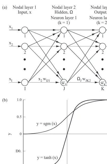
Fig. 1(a) shows a typical two-layer, feed-forward ANN for simulating an input–output response. The ANN consists of two weight layers corresponding to two neuron layers and connecting three nodal layers; the input layer processes no signal, and this layer is not considered to be a neuron layer. Each node is connected to all the nodes in the adjacent layers, and the signal fed at the input layer flows forward layer-by-layer to the output layer. The input layer receives the input vector (record or data), and one neuron is assigned to each input component (field or variable). The output layer generates the output vector, and one neuron is assigned to each output component. Between these two layers, the hidden layer exists and it has arbitrary number of neurons. Notationally, Fig. 1(a) shows an I-J-K ANN, and the nota-tions used are
x¼[x1,x2, …,xI]T (1a)
Q¼[Q1,Q2, …,QJ] T
(1b)
y¼[y1,y2, …,yK] T
(1c)
¯
w¼[w¯1,w¯2, …,w¯jk, …,w¯JþK]
T
(1d)
w¼w1,w2, …,wijk, …,wJ(IþK)]
T
(1e)
where x¼input vector of I components;Q¼hidden vector of J components; y¼ANN output vector of K components;
¯
w¼threshold weight vector of (JþK) components where ¯
wJK ¼threshold of jth neuron in (k þ 1)th neuron layer; and w ¼ weight vector of J(I þ K) components where wijk¼weight connecting ith neuron in kth neuron layer to
jth neuron in (k þ 1)th layer. As such, I and K fix the
numbers of neurons in the input and output layers, and the ANN may be noted to have M¼ ½ðJþKÞ þJðIþKÞÿ
weights where M is the total number of weights. Hecht-Nielsen3suggestion may be used to define an upper limit of J ¼ (2I þ 1) neurons in the hidden layer. Finally, each hidden or output neuron is associated with a transfer func-tion, f(·).
2.3 Operation
In simulating the x–y response for a given x, ANN follows two steps. First, x is fed at the input layer, and ANN
x2
2 2 2
y2
x1
1 1 1
y1
xI
I J K
yK
x2 wIJ1 ΩJ wJK2
wJ1 wK2
(a) Nodal layer 1
Input, x
Nodal layer 2
Hidden, Ω
Neuron layer 1 (k = 1)
Nodal layer 3 Output, y Neuron layer 2
(k = 2)
(b) 1.0
Ð1. 0.5
0
Ð0.
y
Ð Ð Ð Ð Ð 0 1 2 3 4 5
x y = sgm (x)
y = tanh (x)
generatesQas
Second, ANN presentsQto the output layer to generate y as
yj¼f w¯jkþ
whereG(·)¼underlying x–y response vector approximated by ANN; and Gj(·)¼ jth component of G(·). Thus, ANN may be viewed to follow the belief that intelligence manifest itself from the communication of a large number of simple processing elements.7
The transfer function, f(·), is usually selected to be a non-linear, smooth, and monotonically increasing function, and the two common forms are
f(·)¼sgm(·)¼ 1
1þexp(·) (4a)
f(·)¼tanh(·)¼exp(·)¹exp(¹·)
exp(·)þexp(¹·) (4b)
where sgm(·)¼sigmoid function and tanh(·)¼hyperbolic tangent function. Fig. 1(b) shows these functions which are generally assumed to be equally applicable.2
3 ARTIFICIAL NEURAL NETWORK DEVELOPMENT
ANN training is performed to determine the weights, ¯w and w, optimally, and training is performed using an appropriate algorithm. Several algorithms exist to perform the training, and each algorithm is based on one of three approaches: unsupervised training, supervised training, or reinforced training; for example, the Hebbian, back-propagation, and genetic algorithms are based on the unsupervised, super-vised, and reinforced approaches, respectively.12 In the next section, the ANN training procedure and two training algorithms are discussed.
3.1 Training procedure
ANN is developed in two phases: training (accuracy or cali-bration) phase, and testing (generalization or validation) phase. In general, a subset of patterns is first sampled from the domain into a training and testing subset, S, and S is then exhausted by allocating its patterns to a training subset, S1, and a testing subset, S2. The notations
used are
d¼[d1,d2, …,dK] (5a)
S1{(x1,d1), (x2,d2), …, (xP1,dP1)} (5b)
S2¼{(x1,d1), (x2,d2), …, (xP2,dP2)} (5c)
where d ¼ desired output vector of K components corresponding to x; S1¼training subset with P1patterns; and S2¼testing subset with P2patterns. As S2represents the domain partially, testing as a synonym for validation should be viewed with caution.
In the ANN training phase, the objective is to determine the ¯w and w that minimizes a specific error criterion defined to measure an average difference between the desired responses and ANN responses for the P1patterns contained in S1. As such, ANN training becomes an unconstrained, nonlinear, optimization problem in the weight space, and an appropriate algorithm may be used to solve this problem. In the ANN testing phase, the objective is to determine the acceptability of the ¯w and w, thus obtained, in minimizing the same error criterion for the P2patterns contained in S2. As the S2 set is not used in determining ¯w and w, ANN testing assesses domain generalization achieved by the trained ANN and, thereby, builds confidence levels expected from the trained ANN for future predictions. In the next section, the two most commonly used training algo-rithms, back-propagation algorithm (BPA) and genetic algorithm (GA), will be discussed.
3.2 Back-propagation algorithm
Rumelhart et al.7presented the standard BPA, a gradient-based algorithm. Since then, BPA has undergone many modifications to overcome its limitations, and NeuralWare, Inc.12 presents many such modifications. In general, BPA determines ¯w and w in two steps. First, BPA initializes ¯w and w with small, random values. Second, BPA starts updat-ing ¯w and w using S1. During an update from (m¹1) to m (m¼updating index), BPA selects a random integer p[[1, P1] and uses (xp, dp) to minimize the mean squared error equations are written as
wmijk¼w
wherem ¼training rate and y ¼momentum factor. Note y¼0 for m¼1. BPA continues updating ¯w and w until
m¼M, where¯ M is a user-defined number.¯
3.3 Genetic algorithm
Holland20 presented the GA as a heuristic, probabilistic, combinatorial, search-based optimization technique pat-terned after the biological process of natural evolution. Goldberg21 discussed the mechanism and robustness of GA in solving nonlinear, optimization problems, and Montana and Davis22 applied GA quite robustly in ANN training. In general, GA determines ¯w and w in three steps. First, GA samples an initial population of N random configurations of ¯w and w from the weight space defined as
¯
wij[[¹q,þq]q.0 (8a)
wijk[[¹q,þq]q.0 (8b)
whereq¼weight bound. GA encodes each ¯w and w con-figuration in binary strings with Ls bits (Ls ¼ string length) and associates each string with a fitness value defined as
where s¼string index; Fsg¼fitness for sth string after gth generation; Egs ¼mean squared error for sth string after gth generation; ¯wgs¼w in sth string after gth generation;¯ wgs¼w in sth string after gth generation; and y strings with smaller errors. Second, GA starts updating this initial population using S1 for G generations. During an update from (g¹1) to g (g¼generation index), GA per-forms four operations: scaling, selection, crossover, and mutation: (1) GA scales linearly the fitnesses in the (g ¹
1)th population within an appropriate range using a scaling coefficient, C, where C is defined as the number of best strings expected in the scaled population;21(2) GA updates this population by selecting strings with a higher fitness with a higher probability; (3) GA perturbs the resulting population by performing crossover with a probability of pc; and (4) GA further perturbs the resulting population by performing mutation with a probability of pm. As such, GA evaluates N(Gþ1) configurations, and the optimal config-uration is searched from these configconfig-urations.
4 FLOW AND CONTAMINANT TRANSPORT IN THE UNSATURATED ZONE
4.1 Unsaturated flow
In this manuscript, a problem related to flow and transport through a one-dimensional vertical unsaturated soil profile is selected to evaluate the applicability of ANN and to improve the approach. The steady state unsaturated flow equation in one-dimension can be written as
d
where h¼pressure head; Kz¼hydraulic conductivity; z¼ depth measured downward; and Lc ¼column length. The soil–water retention relationship given by the van Genuch-ten parametric model23 is used, and this model can be written as
where Ks ¼ saturated hydraulic conductivity; v ¼ volu-metric water content; vs ¼ saturated water content; vr ¼
residual water content; a ¼grain size distribution index; andbis a curve fitting parameter. The boundary conditions used are a constant steady downward water flux, q, from the profile top and stipulated water pressure head of h¼0, at the profile base. These boundary conditions can be written as
4.2 Single species reactive contaminant transport
The one-dimensional governing equation for transient trans-port of a single species is written as
l¼l1þ
rbk1C
n¹1
v
l2 (14c)
where C ¼ contaminant concentration; D ¼ dispersion coefficient neglecting molecular diffusion;e¼dispersivity; R ¼retardation coefficient; l ¼ overall first order decay coefficient;l1¼dissolved phase, first order, decay coeffi-cient; l2 ¼adsorbed phase, first order, decay coefficient; rb¼soil bulk density; k1¼Freundlich coefficient; and n¼ Freundlich exponent.24The soil profile is initially contami-nant free. The boundary conditions correspond to a steady inflow of a TCE dissolved water pulse from the profile top at C(0,t)¼C0until t¼t0followed by fresh water injection. The profile base is assumed to be under zero dispersive flux condition. These initial and boundary conditions can be written as
C(z,t¼0)¼0 0#z#Lc (15a)
C(0,t)¼C0 t#t0 (15b)
¼0 t.t0
]C
]z
z¼L
¼0 (15c)
5 RESEARCH APPROACH
In this paper, the focus is to study the six research areas identified in a previous section related to the objectives, and the study is performed using simulation of a GFCT model related to flow and transport through a one-dimensional vertical soil profile. Once the base case scenario and related properties are defined, simulations are performed to gener-ate the breakthrough concentration at the profile base for different scenarios, and these simulations are performed using the computer code, HYDRUS.24 Using a selected number of key features of the breakthrough curve (BTC), useful ANN concepts related to architecture, sampling,
training, and multiple function approximation are studied, and the potentials of BPA and GA in ANN training are compared. Finally, a general guideline for simulating GFCT responses using ANN is suggested.
5.1 Base problem: unsaturated zone flow and single species mass transport
The base problem consists of a vertical sandy clay loam profile of 500 cm with a steady water flux of q ¼
10 cm day¹1at the profile top and a steady water table at the profile base. The flow parameters are a ¼0.05 cm¹1; b¼2;vs¼0.4;vr¼0.1; and Ks¼30 cm day
¹1, and the TCE slug consists of a uniform concentration of C0 ¼ 15mg L¹1 for t0 ¼15 days. The remaining properties are e¼1.6 cm;rb¼1.6 gm cm¹3;l1¼0.001 per day;l2¼0; n ¼ 1 (linear Freundlich isotherm); and k1 ¼ 0.293 cm3gm¹1(k1 ¼ kd, the distribution coefficient, for n ¼ 1). Also, to ensure numerical stability and minimal numerical dispersion, Dx¼2 cm (Dx¼space increment) andDt¼0.1 days (Dt¼time step) were used.
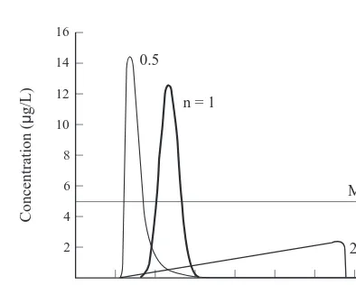
The base problem is solved using HYDRUS for 160 days for n ¼{0.5, 1, 2}, where the base value is n¼1. Fig. 2 shows the three BTCs at the profile base, and it also shows the line corresponding to the maximum contaminant level (MCL) of 5mg L¹1for TCE. Four important features of the BTC are noted. First, as t increases from 0 to 160 days, the concentration increase from zero to maximum to zero. Second, as n increases from 0.5 to 1 to 2, the breakthrough time varies approximately from 23 to 32 to 20 days. Third, as n increases from 0.5 to 1, the time to exceed the MCL of 5mg L¹1varies approximately from 24 to 42 days. When n
¼2, the concentrations remained less than the MCL. Fourth, as n increases from 0.5 to 1 to 2, the maximum concentra-tion varies approximately from 14.5 to 12.5 to 2.5mg L¹1. As such, the BTC is a nonlinear nonmonotonic function of t and n, and the problem appears to be well-defined to pursue the research objective.
5.2 Breakthrough concentration
ANN development for simulating the BTC requires precise identification of the input and output vectors. From eqn (10), the pressure head, h, can be expressed as
h¼h z,Lc,a,b,vs,vr,Ks,q
ÿ
(16)
and from eqn (13), the concentration, C, can be expressed as
C¼C v,t,q,rb,e,l1,l2,k1,n,C0,t0
ÿ
(17)
From eqns (16) and (17), the breakthrough concentration, C*, at the profile base may be expressed as
Cp¼Cp Lc,a,b,vs,vr,Ks,q,t,rb,e,l1,l2,k1,n,C0,t0
ÿ
(18)
In order to reduce the domain, Lc;b,vs,vr,rb,l2, C0, and t0
16
0 12
8
2
Concentration (
µ
g/L)
20 40 60 80 100 120 140 160
Time (days) n = 1
2 0.5
14
10
4
6 MCL
are held constant at the base values, and eqn (18) is reduced to
Cp ¼Cp(F,t,T) (19a)
where
F¼{a,Ks;q} (19b)
T¼{q,e,l1,k1,n} (19c)
where F¼subset of flow parameters; and T ¼ subset of transport parameters. It should be noted that when eqn (18) is simplified to eqn (19), a number of flow and transport parameters, L;b;vs;vr,rb,l2, C0, and t0, are kept constant. This simplification is made to simplify studying the applic-ability of ANN while considering the most significant flow and transport parameters such asaor Ks. Also, the simpli-fication helps to make conclusive remarks on the overall applicability by considering the effects of the few most significant parameters instead of all parameters. In the next section, the applicability of ANN in simulating eqn (19) is assessed.
5.3 Training and testing subset
The flow and transport parameters are allowed to vary over the domain given bya[[0.025, 0.100]; Ks[[15, 60]; q[ [5, 20];e[ [0.8, 3.2];l1[[0.0005, 0.0020]; k1[[0.15, 0.50]; and n[[0.5, 1.0], and the training and testing subset, S, is sampled from this domain. A subset of 100 realizations of x is sampled at random; C*for each realization is deter-mined using HYDRUS, and the 100 patterns are placed in the training and testing subset, S.
5.4 Allocation method
In allocating S to a training subset, S1, and a testing subset, S2, a simple allocation method is applied pattern-by-pattern on S and this method is based on an user-defined expected fraction,f , where˜ f˜[(0,1). In allocating a pattern to S1or S2, a random number r[ (0, 1) is generated. If r#f , the˜ pattern is allocated to S1; otherwise, it is allocated to S2. The sequence of r is simulated using a random number generator initiated by a seed,r, and the allocation method becomes a function off and˜ r. For a given S, the allocation method is expected to allocatef and (1˜ ¹f ) fractions of S to˜ S1 and S2, respectively, and this approach is expected to generate S1and S2of different or similar sizes for different values off and˜ r.
5.5 Artificial neural network development
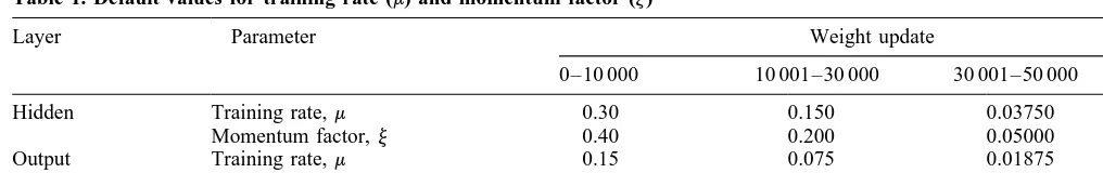
In this manuscript, ANNs are developed using the Neural Works Professional II/Plus, a commercially available soft-ware package.12 The internal parameters of the ANN include initial weight distribution, transfer function, input–output scaling, training rate (m), momentum factor (y), training rule, and the number of weight updates (M).¯ ANN training is performed using the default values in the package, except the seed, r. A common r is used for the allocation method and training for consistency. As such, the initial weights are randomly distributed over [¹0.1, þ0.1]. The transfer function used was sgm(·) or tanh(·). The input–output scaling is performed using the minimum and maximum values of each input and output component contained in S1; the input components are line-arly scaled over [¹1, þ1], and the output components are linearly scaled over [ þ0.2, þ 0.8] or [¹ 0.8, þ0.8] depending on the use of sgm(·) or tanh(·), respectively.12 The default values of m andy are shown in Table 1. The generalized delta training rule for BPA and M¯ ¼50 000 are used. As such, the performance of BPA may be expressed as
h¼h rÿ ,f˜,J
(20)
whereh¼performance of BPA.
5.6 Performance criteria
ANN is trained to approximate a vector function,G(·), and the performances of ANN in approximating each ith component, Gi(·), during training and testing phases need to be assessed. In the ANN training phase, the objective is to match the desired response, di, with the ANN response yi, at each ith output neuron for all the patterns in S1. As such, the performance of training in approximating Gi(·) is assessed using the correlation coefficient defined as
Ri¼
jdiyi
jdijyi
jdi.0; jyi.0 (21a)
j2diþyi¼j 2
d2
i þ2jdiyiþj 2
y2
i (21b)
where Ri¼correlation coefficient between diand yi;jdi ¼ standard deviation of di;jyi¼standard deviation of yi; and
jdiþyi¼standard deviation of (diþyi). Finally, an average performance of the training phase in approximatingG(·) is assessed using the average correlation coefficient, R, Table 1. Default values for training rate (m) and momentum factor (y)
Layer Parameter Weight update
0–10 000 10 001–30 000 30 001–50 000
Hidden Training rate, m 0.30 0.150 0.03750
Momentum factor,y 0.40 0.200 0.05000
Output Training rate, m 0.15 0.075 0.01875
defined as
In addition, the performance of training is assessed using scatter plots of yiversus di, and the scatter ofðdi, yi) from the 458line is assessed using two error bounds defined as
ya¼(1¹e)d (23a)
yb¼(1þe)d (23b)
where e ¼ specified error in decimal values; ya¼ lower error bound corresponding to e; and yb¼upper error bound corresponding to e. A scatter plot helps to assess ANN performance more effectively compared to R. In the ANN testing phase, the objective is to match diwith yiat each ith output neuron for all the patterns in S2. As such, the performance of testing in predictingG(·) is assessed by repeating the above procedure for S2.
6 ARTIFICIAL NEURAL NETWORK ASSESSMENT
Several example scenarios related to the GFCT model are solved to assess the ANN applicability. In general, the accu-racy of ANN training is observed to be approximately 100%, and the generalization of ANN testing is observed to limit the applicability of ANN. In the next section, the applicability of ANN with respect to only ANN testing is discussed.
6.1 Example 1: simulation of the BTC with linear adsorption
ANN was used to simulate the breakthrough concentration, C*, with n ¼1 (Fig. 2). C* is a nonlinear nonmonotonic function of time, t, and helps to assess the applicability of ANN in simulating such a function. As the input is only time (I¼1), a hidden layer of three neurons (J¼3) was used,3 and a 1-3-1 ANN was used to simulate C*. In predicting C* for 160 days, HYDRUS generates 1618 patterns of (C*, t); these patterns are included in the training and testing subset,
S, and the allocation method was used for allocating S to S1
and S2. As no guideline for the allocation exists,f˜¼0:5 was used to minimize bias on the allocation, and r ¼ 1 was arbitrarily taken.
Fig. 3 shows the predicted C*when ANN is trained using sgm(·). The results show that ANN fails to simulate C* correctly. In order to improve the ANN performance, attempts were made to train the ANN with f˜ ¼ {0.25, 0.75},r¼{5, 257}, and J¼{15, 30}; yet, the performance did not improve. Thereafter, ANN was trained using tanh(·) as the transfer function. The results in Fig. 3 show that the performance of ANN improves dramatically, and the ANN induced small errors in the breakthrough time and maximum concentration. Fig. 4 shows the scatter plot for desired (HYDRUS) and predicted (ANN) responses, and R ¼
0.995 where R is the correlation coefficient. Although R is high, a few large errors are observed for C#3mg L¹1, and errors of 10–12% are observed for C.3mg L¹1. As such, R alone appears not to be a robust index for assessing the performance of ANN, and scatter plots with appropriate error bounds are needed to assess the performance robustly. Finally, the sensitivity of the ANN tof˜¼{0.25, 0.5, 0.75}, r¼{1, 5, 257}, and J¼{3, 15, 30} were analyzed, and the corresponding R values are observed to vary over R [ [0.994, 0.998]. Although not shown here, these results sug-gested that ANN is insensitive to these parameters for the present example.
As sgm(·) and tanh(·) are considered equally applicable,2 the present example suggests that these two functions may be regarded as complementary. In cases where one function fails to perform robustly, the other may be used. Also, a careful examination of these results reveal one important aspect of ANN training. C* is mostly small within the 160 days, except near the peak concentration times, and this may have caused the poor performance of sgm(·).12 Both sgm(·) and tanh(·) are s-shaped functions, but they 16
Fig. 3. Breakthrough concentration of Example 1 with linear adsorption using HYDRUS and 1-3-1 ANN with two different
transfer functions
Desired concentration (µg/L)
Ð20 Ð10 +10%
differ in their output ranges (Fig. 1(b)). The output range of sgm(·) is (0, 1) while the output range of tanh(·) is (¹1,
þ1). As BPA uses the output of a transfer function as a multiplier in the weight update, sgm(·) produces a small multiplier when the summation is small, and vice versa. Therefore, there is a bias towards training higher desired outputs. In contrast, tanh(·) produces equal multipliers when the summation is either small or large and, therefore, tanh(·) leads to no bias towards training lower or higher desired outputs.
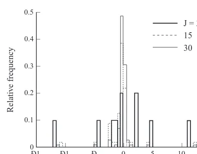
The ANN results are further studied to determine the effect of the number of hidden nodes on the weight distribu-tion. Fig. 5 shows the weight histograms of 1-J-1 ANN for J¼{3, 15, 30}, and the weights are observed to decrease with increasing J. As J is increased, more terms are consid-ered in the argument of a output neuron (eqn (2b)), and its weighted sum becomes very small or large if the weights do not decrease. At a very small or a large sum, the output of a transfer function is essentially independent of the sum (Fig. 1(b)), and the ANN may fail to approximate the input– output response robustly. As such, BPA decreases weights with increasing J to train the ANN robustly and makes ANN insensitive to J over a wide range. However, this observa-tion contradicts recent observaobserva-tions by others suggesting
poor ANN testing with increasing J beyond an optimal value.4-5As such, the present example suggests that ANN is sufficiently, but not completely, insensitive to J around the optimal value.
6.2 Example 2: simulation of BTC with nonlinear adsorption
In the previous example, the applicability of ANN in pre-dicting C*was studied when the mass transport simulation is simple due to linear solid phase adsorption. In the present example, the applicability of ANN in predicting C* is studied when the mass transport is complicated due to non-linear solid phase adsorption. As such, ANN is attempted to simulate C*with n¼{0.5, 1, 2} (Fig. 2). In this case, C*is a nonlinear nonmonotonic function of continuous t and dis-crete n, and helps to assess the applicability of ANN in simulating such a function. As the inputs are only t and n (I ¼2), a hidden layer of five neurons (J¼5) is used,3 and a 2-5-1 ANN is used to simulate C*. In predicting C*for 160 days, HYDRUS generated a total of 5405 patterns of (C, t, n). These patterns are included in S, and the allocation method withf˜¼0.5 andr¼1 was used for allocating S to S1 and S2. The ANN is trained using the tanh(·) transfer function.
Fig. 6 shows the predicted C*, and the results show that ANN failed to predict C*satisfactorily. For n¼{0.5, 1.0}, ANN introduces large errors in the predicted spread and maximum concentration and predicts the desired responses qualitatively. However, for n¼2, ANN prediction is poor both qualitatively and quantitatively. In the present exam-ple, C* varies more rapidly with t than with n, and ANN finds it difficult to cope with these different paces of variations. In order to improve the robustness of ANN, the sensitivity of ANN tof˜¼{0.25, 0.5, 0.75},r¼{1, 5, 257}, and J ¼ {3, 5, 10} were analyzed, and the results are summarized in Table 2. For f˜ ¼ {0.25, 0.5, 0.75}, ANN performance increases with increasing f . As˜ f increases,˜ ANN receives more patterns for training, acquires a clearer picture of the domain, and improves its generalization. For r¼{1, 5, 257}, ANN performance is intermediate forr¼1, worst forr ¼5, and best forr ¼257. Asr varies, ANN acquires different weight configurations due to the 0.5
0 0.4
0.1
Relati
v
e frequenc
y
Ð1 Ð1 Ð 0 5 10 15
0.3
0.2
Weight
J = 3 15 30
Fig. 5. Weight histogram of 1-J-1 ANN for predicting the break-through concentration of Example 1
16
12
8
2
Concentration (
µ
g/L)
0 20 40 60 80 100 120 140 160
Time (days)
ANN Hydrus
14
10
4
6 MCL
n = 1 0.5
2
Fig. 6. BTC of Example 2 using HYDRUS and 2-5-1 ANN with different n values
Table 2. Sensitivity of 2-5-1 ANN to expected fraction (f ), seed˜ (r), and hidden nodes (J) for Example 2
˜
f r J R
0.25 1 5 0.875
0.50 1 5 0.896
0.75 1 5 0.914
0.50 1 5 0.896
0.50 5 5 0.867
0.50 257 5 0.901
1 0.50 3 0.867
1 0.50 5 0.896
entrapment of BPA at different local optimal solutions. For J¼{3, 5, 10}, ANN performance increases with increasing J. As J increases, ANN acquires more freedom for approximating C*. Also, this observation suggests that
Jopt.10.JHN ðJopt¼J at optimal performance and
JHN¼J recommended by Hecht-Nielsen
3
) for the present example.
In investigating this problem, an interesting phenomenon is noted; i.e. t is changing more rapidly than n. In these scenarios, t is the primary, independent variable and is sup-posed to change more rapidly compared to other parameters such as n, and the weights may fail adjusting to these inputs with disproportionate variations. Although this problem may be handled to some extent by increasing J, this approach will lead to larger ANN, a larger optimization problem, and a greater difficulty in training. Alternatively, an innovative ANN architecture may be considered. Instead of simulating C*as a continuos function of t, ANN may be used to simulate C*as a discrete function of time. Notation-ally, the continuous function, C*¼C*(t, n), may be replaced by the discrete function, C*¼{C*(ti, n), i¼1, 2,.., T}, and an 1-3-T ANN may be used to simulate this discrete func-tion. As such, t is distributed across the output layer, and this approach resembles the concept of distributed input–output representation.
6.3 Example 3: use of ANN to simulate BTC parameters
In the previous example, an innovative ANN architecture based on the concept of distributed input–output represen-tation is introduced to simulate C*¼C*(t, n). In the present example, this innovative architecture is implemented. In typical groundwater remediation problems, the four key parameters of the BTC are (1) breakthrough time, tb; (2) time to reach MCL, tMCL; (3) time to maximum concentra-tion, tmax; and (4) maximum concentration, Cmax. If one can predict these four values, the prediction of the remaining point values of C*can be avoided.
In the present example, the applicability of the innovative ANN in simulating the four key parameters of the BTC is assessed. These values are considered to be functions of flow parameters, F, and transport parameters, T, defined by eqns (19b) and (19c), respectively. The ANN application is divided into three parts: (1) effect of F; (2) effect of T; and (3) combined effect of F and T. In general, as there are seven inputs (I¼7) and four outputs (J¼4), a 7-J-4 ANN is used, and J is determined, depending on the number of active input components. In studying the effect of F or T, the respective input components in T or F are held constant at base values. However, this condition should not change the
Ð5
100
80
20
Predicted t
b
(days)
0 20 40 60 80 100
40 60
Desired tb (days)
(a)
Ð5
100
80
20
Predicted t
MCL
(days)
0 20 40 60 80 100
40 60
Desired tMCL (days)
(b)
+5%
+5%
Ð5
100
80
20
Predicted t
max
(days)
0 20 40 60 80 100
40 60
Desired tmax (days)
(c)
Ð5
16
14
2
Predicted C
max
(
µ
g/L)
0 2 8 12 14 16
4 12
Desired Cmax (µg/L)
(d)
+5%
+5%
6 8 10
4 6 10
results since ANN considers a constant input component to be a threshold weight, and ANN training adjusts other weights to take this into account. In the next section, a subset of 100 realizations is sampled at random and C*for each realization is determined using HYDRUS. Thereafter, the 100 patterns are placed in the corresponding training and testing subset, S. The allocation method withf˜ ¼0.5 and r¼1 is then used for allocating S to S1 and S2. ANN used tanh(·) as the transfer function and trained using BPA. At this stage, it may be noted that S of the present example is much smaller than those of the previous two examples.
6.4 Effect of flow parameters
ANN is used to simulate the effect of F on the four key parameters of the BTC. Since there are three active input components in F, a hidden layer of seven neurons (J¼7) was used to construct the 7-7-4 ANN.3 S is sampled at random from the domain given bya[ [0.025, 0.100], Ks
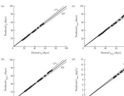
[[15, 60], and q[[5, 20]. Fig. 7(a) shows the result for tb, where R¼ 0.999. The errors of predicting tbwere within
65% for a few patterns. Similarly, Fig. 7(b–d) shows the results for tMCL, tmax, and Cmax, respectively, where R ¼ 0.999 for all these cases and the errors were within 65%. As the ANN is trained using input–output values scaled over a common range, the ANN is not showing a bias towards any particular response. ANN is maintaining an average error for all the functions, and eqn (22) yields the average R ¼0.999. Thus, the results suggest that the innovative ANN architecture can accurately simulate the effect of F on the four key parameters of the BTC and can overcome the poor results of the previous example where the prediction of the entire BTC was attempted.
The sensitivity of the ANN tof˜¼{0.25, 0.50, 0.75},r¼
{1, 5, 257}, and J¼{4, 7, 14} were studied, and the corre-sponding R values varied over R [ [0.98, 1]. f˜ ¼ 0.25 produced the minimum R due to inadequate representation of S in S1, andrand J did not have any effect on R.
6.5 Effect of transport parameters
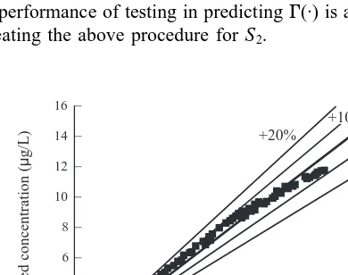
In this section, ANN was used to simulate the effect of T in predicting the key features of the BTC. Since there are five active input components in T, a hidden layer of 11 neurons (J ¼ 11) was used to construct the 7-11-4 ANN.3 S is sampled from the domain given by q[ [5, 20],e[[0.8, 3.2],l1[[0.0005, 0.0020], k1[[0.15, 0.60], and n[[0.5, 1.0]. Fig. 8 shows the result for Cmaxwhere R¼0.985. The errors of prediction were mostly within 6 5% and a few maximum errors of 6 15% were observed. Although not shown here, the results of other three parameters showed comparable accuracy. Once again, the results suggest that the innovative ANN architecture can robustly simulate the effect of T. However, it should be noted that ANN is more adaptable to F than to T. One possible reason is that C*is probably a more regular function of F compared to T, and thus, ANN requires less patterns to generalize the response to F than to T.
The sensitivity of the ANN tof˜¼{0.25, 0.50, 0.75},r¼
{1, 5, 257}, and J¼{6, 11, 22} were also studied. Although not shown here, the corresponding R values varied over R[ [0.969, 0.997], and these high R values indicate negligible sensitivity of ANN to these parameters.
6.6 Effect of combined flow and transport parameters
In this section, ANN was used to simulate the combined effect of F and T on the BTC parameters. Since there are seven active input components in combined F and T, a hidden layer of 15 neurons (J¼15) was used to construct the 7-15-4 ANN.3S is sampled from the domain given bya
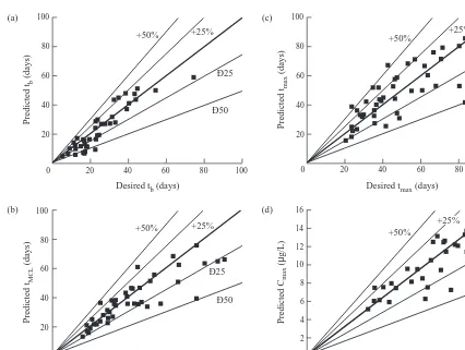
[[0.025, 0.100], Ks[[15, 60], q[[5, 20],e[[0.8, 3.2], l1[[0.0005, 0.0020], k1[[0.15, 0.60], and n[[0.5, 1.0]. Fig. 9(a) shows the result for tb, where R¼0.997. The errors were mostly 610%, and the maximum errors were 625% on few occasions. Fig. 9(b,c) shows the testing results for tMCLand tmaxrespectively, where for both these cases R¼ 0.999 and the errors stayed within 610%. Fig. 9(d) shows the results for Cmax, where R¼0.998, and the errors were within 615%. As discussed previously, ANN did not show a bias towards any particular response and ANN is main-taining an average error for all the functions. For this case, eqn (22) produced an average R¼0.998. Also, when Figs 8 and 9(d) are compared, it is seen that two figures are almost similar. The errors in the four key parameters of the BTC are primarily due to the effect of T. Therefore, these results suggest that the innovative ANN architecture can accurately simulate the effect of combined F and T and can overcome the poor results of the previous approach.
Finally, the sensitivity of the ANN to f˜ ¼{0.25, 0.50, 0.75},r¼{1, 5, 257}, and J¼{8, 15, 30} were studied. As in the previous section, the corresponding R values varied over R[ [0.896, 0.993], and these high R values indicate negligible sensitivity of ANN to these parameters.
16
12
8
2
Predicted C
max
(
µ
g/L)
0 2 4 6 8 10 12 14 16
+15%
14
10
4 6
Desired Cmax (µg/L)
Ð15 +5% Ð5
7 GENETIC ALGORITHM
In the previous sections, ANN training of all the examples was performed with relatively high accuracy using BPA. In general, ANN training is an unconstrained, nonlinear, opti-mization problem. It is plagued with local optimum. In some situations, the gradient-based BPA may become trapped at a local optimal solution, and consequently, ANN training may
suffer. Alternatively, ANN training may be performed using GA. The search-based GA can avoid becoming trapped to a local optimal solution, and it can be used in situations where BPA fails. Montana and Davis22 robustly applied GA to train an ANN, and the research showed that GA can be used as an alternate technique when BPA fails. In the next section, GA is used to train the 7-15-4 ANN to simulate the effect of combined F and T on the key parameters of the BTC. A set of 100 realizations was sampled at random from the domain given bya[[0.025, 0.100], Ks[[15, 60], q [ [5, 20],e[ [0.8, 3.2],l1 [ [0.0005, 0.0020], k1 [ [0.15, 0.60], and n[ [0.5, 1.0]. C*for each realization is determined using HYDRUS, and the 100 patterns were placed in the training and testing subset, S. Thereafter, the allocation method with f˜ ¼0.5 and r ¼ 1 was used for allocating S to S1and S2. ANN used tanh(·) as the transfer function and was trained using GA. In the next paragraph, the applicability of GA in ANN training is assessed.
GA requires a weight space to search for optimal weights. Fig. 5 suggests that q ¼0.5 may be assumed to train an ANN with J ¼ 15, and eqn (8) was used to define the weight space as wi[[¹0.5, þ0.5] (wi¼ith component of w, and w ¼weight vector containing all w¯ij and wijk). Next, standard GA is implement to determine the optimal weights with C, pc, and pm of 2, 0.6, and 0.033, respec-tively.21,25An initial population of 30 strings was sampled at random from this weight space, and the population was 100
80
20
Predicted t
b
(days)
0 20 40 60 80 100
40 60
Desired tb (days)
(a)
Ð10
100
80
20
Predicted t
MCL
(days)
0 20 40 60 80 100
40 60
Desired tMCL (days)
(b)
+10%
Ð10
100
80
20
Predicted t
max
(days)
0 20 40 60 80 100
40 60
Desired tmax (days)
(c)
Ð15
16
14
2
Predicted C
max
(
µ
g/L)
0 2 8 12 14 16
4 12
Desired Cmax (µg/L)
(d)
+10%
+15%
6 8 10
4 6 10
+25%
Ð25 Ð10 +10%
Fig. 9. Performance of 7-15-4 ANN in Example 3: (a) breakthrough time; (b) time to reach MCL; (c) time to reach maximum concentration; and (d) maximum concentration
taken through 100 generations. In Fig. 10, the heavy line shows the mean squared error at any generation, and ANN training performance is observed to be poor. In order to improve ANN training, an alternate GA is used and the procedure involved can be described as follows:
1. the initial population of 30 strings was taken through 10 generations. Then, the best solution, w1, is identi-fied, and it is assumed to be in the global–optimal region;
2. w1is updated locally and a small space around w1is defined as wi[½wli¹2qj, wliþ2qj]ðwli¼ith com-ponent of w1). A j value of 0.15 was arbitrarily assumed. An initial population of 30 strings is sampled from this weight space, and the population was taken through nine generations. From the 10 generations thus obtained, the best solution, w2, is identified; and
3. the second step is repeated eight times taking the original initial population through 100 generations; each time, a new weight space is defined around the best solution from the previous time.
The light line in Fig. 10 shows the mean squared error, as defined by eqns (9a) and (9b), at any generation, and ANN training is observed to improve dramatically with the pro-posed GA scheme. In Fig. 10, the dark square shows the best
solution determined by the alternate GA which is at the 89th generation. The corresponding R values varied over R [ [0.853, 0.908] in training. Fig. 11(a–d) shows the corre-sponding results for tb, tMCL, tmax, and Cmax, respectively, in testing. R values for these parameters varied over R [ [0.765, 0.920]. The corresponding scatter plot errors were mostly within 6 25%, and a few maximum errors were within 6 50%. Finally, when Fig. 9(a–d) is compared with Fig. 11(a–d), alternate GA is found to be inferior to BPA. However, these results are not sufficient to produce conclusive evidence to indicate GA is inferior to BPA in ANN applications. These results were based on a single set of simulations, and therefore, more research is needed to prepare alternate GA as a complementary to BPA for situa-tions where BPA may fail.
8 CONCLUSIONS
In solving the present problems, ANN applications appear simple and robust. A small subset of the GFCT responses to hydrogeologic condition and hydrodynamic stimuli needs to be simulated using the numerical GFCT model, and these responses to the remaining conditions and stimuli may be obtained using ANN with simplified computations. Also, the solutions help to address some research issues 100
80
20
Predicted t
b
(days)
0 20 40 60 80 100
40 60
Desired tb (days)
(a)
Ð25
100
80
20
Predicted t
MCL
(days)
0 20 40 60 80 100
40 60
Desired tMCL (days)
(b)
+50%
Ð50
100
80
20
Predicted t
max
(days)
0 20 40 60 80 100
40 60
Desired tmax (days)
(c)
Ð25
16
14
2
Predicted C
max
(
µ
g/L)
0 2 8 12 14 16
4 12
Desired Cmax (µg/L)
(d)
6 8 10
4 6 10
+50%
Ð25 +25%
Ð50
+25%
Ð50
Ð25 +25% +50%
+25% +50%
Ð50
related to such applications, and the following conclusions are made.
1. ANN shows difficulty in considering independent variables such as time as an input. To overcome this problem, an innovative ANN architecture based on the concept of distributed input–output representation appears effective for solving the present problems. 2. ANN training can be performed robustly using BPA,
and ANN testing shows difficulty in generalization. A robust sampling technique is required to represent key features of the domain with fewer patterns. In solving the present problems with training and testing sets sampled at random, ANN training with very high accuracy is achieved using BPA, and ANN testing is observed to limit ANN application.
3. The sigmoid and hyperbolic tangent functions are con-sidered to be complementary; if one fails, the other may be used. Although complementary, the sigmoid function appears less effective than the hyperbolic tangent func-tion for solving the present problems.
4. ANN is observed to be robust for approximating mul-tiple functions. A single ANN appears effective in simulating several key features simultaneously for the present problems.
5. Hecht-Nielsen3suggestion may be used for fixing the number of hidden neurons, J. Although recent research suggest the existence of an optimal J, ANN appears sufficiently, but not completely, insensitive to Hecht-Nielsen’s J for solving the present problems. 6. Alternate GA may be developed as a complementary
to BPA. Although alternate GA performs less robustly than the BPA for solving the present problems, it does show potential for future development.
REFERENCES
1. McCulloch, W. S. and Pitts, W. A logical calculus of the ideas imminent in nervous activity. Bulletin of Mathematical Biophysics, 1943, 5, 115–133.
2. Beale, R. and Jackson, T., Neural Computing: An Introduc-tion. Adam Hilger, Techno House, Bristol, 1991.
3. Hecht-Nielsen, R., Kolmogorov’s mapping neural network existence theorem. In 1st IEEE International Joint Confer-ence on Neural Networks. Institute of Electrical and Electro-nic Engineering, San Diego, 1987, pp. 11–14.
4. Ranjithan, S. J., Eheart, J. W. and Garrett, J. H. Jr. Neural network based screening for groundwater reclamation under uncertainty. Water Resources Research, 1993, 29(3), 563– 574.
5. Rogers, L. L. and Dowla, F. U. Optimization of groundwater remediation using artificial neural networks with parallel solute transport modeling. Water Resources Research, 1994, 30(2), 457–481.
6. Rogers, L. L., Dowla, F. U. and Johnson, V. M. Optimal field-scale groundwater remediation using neural networks and the genetic algorithm. Environmental Science and Tech-nology, 1995, 29(5), 1145–1155.
7. Rumelhart, D. E., McClelland, J. L. and the PDP Research Group, Parallel Distributed Processing: Explorations in the Microstructure of Cognition, Vol. 1. MIT Press, Cambridge, MA, 1986.
8. Voss, C. I., A finite-element simulation model for saturated– unsaturated, fluid-density-dependent groundwater flow with energy transport or chemically reactive single-species solute transport. US Geological Survey Water Resources Investiga-tions, 84-4369, 1984.
9. Johansson, E. M., Dowla, F. U. and Goodman, D. M. Back-propagation learning for multi-layer feed-forward neural net-works using the conjugate gradient method. International Journal of Neural Systems, 1992, 2(4), 291–301.
10. Jang G., Dowla, F. and Vemuri, V., Application of neural networks for seismic phase identification. In IEEE Joint Con-ference on Neural Networks. IEEE, Singapore, 1991. 11. Weigend, A. S., Rumelhart, D. E. and Huberman, B. A.,
Generalization by weight-elimination with application to forecasting. In Advances in Neural Information Processing, Vol. 3, eds R. P. Lippmann, J. Moody and D. S. Touretzky. Morgan Kaufmann, San Mateo, CA, 1991, pp. 395–432. 12. NeuralWare, Neural Computing, NeuralWorks Professional
II/Plus and NeuralWorks Explorer. NeuralWare, Pittsburgh, 1991.
13. Hebb, D., The Organization of Behavior. John Wiley, New York, 1949.
14. Rosenblatt, F. The perceptron: a probabilistic model for information storage and organization in the brain. Psycho-logical Review, 1958, 65, 386–408.
15. Widrow, B. and Hoff, M. E. Adaptive switching circuits. IRE WESCON Conv. Rec., 1960, 4, 96–104.
16. Minsky, M. and Papert, S., Perceptrons. MIT Press, Cambridge, MA, 1969 (expanded edition, MIT Press, Cambridge, MA, 1988).
17. Le Cun, Y. Une precudure d’apprentissage pour re´seau a` seuil assymetrique (A learning procedure for asymmetric threshold network). Proceedings of Cognition, 1985, 85, 599–604.
18. Parker, D. B., Learning-logic. Technical Report TR-47, Center for Computational Research in Economics and Management Sciences, Massachusetts Institute of Tech-nology, Cambridge, 1985.
19. Werbos, P., Beyond regression: new tools for prediction and analysis in behavioral sciences. PhD dissertation, Harvard University, Cambridge, MA, 1974.
20. Holland, J. H., Adaptation in Natural and Artificial Systems. University of Michigan Press, Ann Arbor, MI, 1975. 21. Goldberg, D. E., Genetic Algorithms in Search, Optimization,
and Machine Learning. Addison-Wesley, Reading, MA, 1989.
22. Montana, D. J. and Davis, L., Training feedforward neural networks using genetic algorithms. In Proceedings of the 11th International Joint Conference on Artificial Intelli-gence, Vol. 1. Morgan Kaufmann, San Mateo, CA, 1989, pp. 762–767.
23. van Genuchten A closed-form equation for predicting the hydraulic conductivity of unsaturated soils. Soil Science Society of America Journal, 1980, 44, 892–898.
24. Kool, J. B. and van Genuchten, M. Th., HYDRUS, One-dimensional variable saturated flow and transport model including hysteresis and root water uptake. Research Report No. 124, US Salinity Laboratory, USDA, ARS, Riverside, CA, 1991.