Intangible Investment, Debt Financing and
Managerial Incentives
Michael H. Anderson and Alexandros P. Prezas
We analyze how debt affects a firm’s decision to allocate limited resources between real and intangible assets. Real assets provide cash flows for debt service and collateral in the event of default, while intangibles have a higher net present value which is captured only if debt is repaid. To avoid bankruptcy and the associated loss of the intangible assets’ cash flows, management may be induced to devote more effort in operating the firm, thereby increasing the productivity of the real assets. Alternatively, given debt, investment in intangibles acts to indirectly increase the value of the real assets to bondholders and so reduce the promised debt repayment. Hence, increasing debt financing exogenously may increase investment in intangible assets. © 1999 Elsevier Science Inc.
Keywords: Resource allocation; R&D; Incentive conflict JEL classification: G31, G32
I. Introduction
It is widely accepted that intangible assets, such as R&D or advertising, support less debt than real assets, such as plant and equipment. As intangibles have value only as part of a going concern, this follows from the prediction made by Myers (1977) that the debt-to-value ratio will be lower the larger the proportion of firm debt-to-value represented by investment options. Smith and Watts (1992) provided empirical support to Myers’ claim, while Bradley et al. (1984), and Long and Malitz (1985) supported the argument that increasing the proportion of assets invested in advertising and R&D reduces the borrowing capacity of the firm. It is also widely recognized that, in addition to their disparate debt capacity, the cash flow patterns of intangible and real assets differ in terms of timing and risk. On average, real asset investment starts generating cash flows earlier than intangible asset
Department of Accounting and Finance, Charlton College of Business, University of Massachusetts-Dartmouth, North Massachusetts-Dartmouth, MA (M.H.A.) Department of Finance, Sawyer School of Management, Suffolk University, Boston, MA (A.P.P.).
Address correspondence to: Dr. A. P. Prezas, Department of Finance, Sawyer School of Management, Suffolk University, 8 Ashburton Place, Boston, MA 02108.
investment. However, when successful, intangibles can be expected to generate higher cash flows than comparable investment in real assets.
Another strand of the literature stresses the importance of managerial incentives in the presence of debt financing. For example, Myers (1977) showed how the asymmetry of payoffs between equity and debt holders can induce underinvestment. Jensen and Meck-ling (1976) showed how debt financing can act to control the incentive to overconsume perquisites, mitigating a conflict between inside- and outside-equity holders. In a princi-pal/agent framework, Grossman and Hart (1982) showed how the threat of bankruptcy can (partially) align the manager’s investment incentives with those of owners. Practitioners are also becoming increasingly aware of the need to account for the role managerial incentives play in financial contracting, even in the absence of debt financing. One example occurs in biotechnology, where R&D represents a very significant proportion of total investment but is, at the same time, extremely risky. To align incentives between investors and firm management sufficiently to raise the required funds, SWORD financing was created.1
The purpose of this paper is to examine the impact managerial incentives have on a firm’s decision to allocate funds between real and intangible assets in the presence of debt. In doing so, we assume that managerial action (effort) can influence a project’s payoff, and we analyze managers’ incentives to provide effort. To focus on these effects, we abstract from other types of incentive problems, e.g., owner/manager conflicts. In addi-tion, our approach differs from the existing literature in that we determine investment in intangibles given the debt level, instead of determining debt given the level of intangible investment.
The intuition of the paper is the following. Consider a firm with limited resources, a fixed portion of which is financed with risky debt maturing before the cash flows from intangible assets are realized. The allocation of resources between real and intangible assets is shaped by two competing effects. First, compared with real assets, an equal investment in intangible assets has a higher net present value if the firm continues as a going concern. By itself, this effect causes management to shift more resources to intangibles. Second, as debt is paid from real asset cash flows, less investment in real assets increases the probability that the firm will not survive as a going concern. This effect causes management to devote more effort in operating the firm, thereby increasing the productivity of the real assets, in order to avoid bankruptcy and the associated loss of intangible value. In other words, investment in intangibles may act via effort to indirectly increase the value of the real assets to bondholders and, thus, lower the promised debt repayment. This collateral-like aspect of intangibles has not previously been examined in the literature.
Shifting resources from real to intangible assets is costless, as it does not entail raising additional funds. Hence, given debt, optimal investment in intangible assets is reached when the net impact of the two competing effects on equity cash flows vanishes. Accordingly, exogenous changes in debt affect optimal investment in intangible assets. Given the collateral-like aspect of intangibles, it is shown that higher levels of debt
1SWORD (stock warrant off-balance-sheet R&D) financing is all-equity and used to raise initial funding
financing could be associated with increased investment in intangible assets. This happens when the higher investment in intangibles raises effort and reduces debt repayment, thereby increasing the probability that the firm continues as a going concern and so captures the benefits of its investment in intangible assets.
Our results imply that firm characteristics, specifically capital structure, affect invest-ment in intangible assets like R&D. A testable hypothesis resulting from our analysis is that risky debt financing and investment in intangibles are inversely related if the effort management exerts in operating the firm is inversely related with investment in intangi-bles; otherwise, they could be positively related. Effort in this hypothesis can be proxied by the expenditures on the development of industrial processes—instituted to enhance productivity and/or enable the firm to capture the benefits of being the first on the market with new products resulting from the R&D investment. Caravatti (1992) indicated that such expenditures vary across industries and are higher for Japanese than U.S. firms. Hence, although such expenditures were not considered in their analysis, the finding by Bhagat and Welch (1995) that the relation between last year’s debt ratio and current R&D spending is significantly negative (positive) for U.S. (Japanese) firms provides indirect support for our hypothesis.
Our paper also relates to the existing empirical literature which examines the equity pricing implications of R&D investment. Chan et al. (1990), Doukas and Switzer (1992), and Zantout and Tsetsekos (1994) detected statistically significant stock price increases in response to announcements of increased R&D expenditures. Further, Zantout (1997) found that the positive stock-price reaction to new R&D expenditures is more pronounced for firms employing more debt in their capital structure. He interpreted this as providing support for the debt-monitoring hypothesis discussed in Grossman and Hart (1982), Jensen (1986), Harris and Raviv (1990) and Stulz (1990). Our findings provide a potential justification for the Zantout (1997) choice of R&D, as opposed to any type of capital expenditure, in testing this hypothesis. In our model, the positive relationship between debt financing and investment in intangibles like R&D results from the manager’s increased effort in an attempt to avoid bankruptcy and capture the cash flows of the intangible assets. Stepped-up effort results in a more economically viable investment, and so equity value increases.
The layout of the paper is as follows. The next section describes the basic model. Section III considers the owner’s effort problem, while Section IV considers the debt-pricing problem. Section V considers the investment allocation problem and its compar-ative statics, as well as a special case. Conclusions follow in Section VI. The model’s notation is summarized, and proofs are gathered in the Appendix.
II. The Model
produces only a t 5 2 cash flow and has zero salvage value at any date.2 As we are interested in the trade off between these technologies, we assume that the sum of the investment levels is constant and normed to one unit of funds. We assume universal risk-neutrality, a competitive debt market and, for notational simplicity, a zero discount rate.
At t50, the owner decides the proportion of total investment, x[[0, 1], to be put into current production, the remainder goes into intangibles.3Also, at t50, the owner raises an exogenous amount, B, in debt financing, the remainder, 12B, represents equity. After the investment allocation decision is made and the debt is priced, the owner chooses an effort level, e$0, which impacts the project’s cash flows.4Effort is costly to the owner; as is standard, we assume that this cost is convex and increasing in effort. To simplify the analysis, we adopt a quadratic form for this cost. Note that the effort decision is made after investment is chosen; however, to avoid an overly complicated model chronology, we label it as a t5 0 decision.
Cash flows are random and depend on exogenous uncertainty, the level of investment and the effort choice. For current production, cash flows at t51 and t52 are independent and identically distributed, each given by p˜C( x, e), where p˜ is a random component described by a c.d.f. F( p˜), and C[is a non-random component. The t51 salvage value of current production,D, is taken to be a proportion,d[[0, 1], of the expected t52 cash flow, i.e.,D [dE( p˜)C( x, e). In foreclosure, assets lose value because of inefficiencies in liquidating them and/or because a portion of their value is firm-specific. Consequently, the greater the assets’ redeployability, the greater the portion of value recovered in a foreclosure/liquidation, and so the higher isd.
For intangibles, the t 52 cash flow is given by q˜D(12 x, e), where q˜ is a random component described by a c.d.f. G(q˜), and D[ is a non-random component. As it is understood that p˜ and q˜ are random, we henceforth suppress tildes. To simplify mathe-matical exposition, we assume p and q are uniformly distributed over the intervals, [0, p#] and [0, q#], respectively; p#, q#.0. Further, C[uxe and D[f(12x)e;u,f.0.5With this parameterization, a necessary condition for intangibles to be more attractive to the firm, relative to current production, is:
q#f .2p#u. (1)
This condition says that for a given level of investment, y, and effort, e, the expected return from intangibles exceeds that from current production, i.e., E(q) D( y, e) .
2We assume zero salvage value for mathematical tractability; however, all that is required is a lower t51
salvage value for intangibles relative to tangibles, given equal investment. Further, our modeling of intangibles is in line with recent work in the economic literature, e.g., Rosen (1991) and Quirmbach (1993).
3Our analysis is complementary to Myers (1977). Specifically, he considered whether future investment will
proceed given a fixed allocation between “assets in place” and “PVGO”, while we consider how, given an investment opportunity set, such an allocation is chosen.
4Effort can be viewed as encompassing a variety of activities enhancing profitability or franchise value
aimed at customers, vendors, workers or others in the firm’s nexus of contracting relationships; for instance, increasing perceived customer satisfaction, enhancing worker productivity, improving the quality of a vendor’s inputs, or accelerating the transformation of R&D concepts into new products.
5The main conclusion reached in this paper about the relation between debt financing and investment in
2E( p)C( y, e) (recall that the former produces only one cash flow while the latter has two). In other words, for given investment and effort, intangibles have a higher net present value than current production. On the other hand, under these conditions, R&D is riskier, i.e., has greater variance, than does current production.6
Given positive t50 borrowings, B, the owner will owe Bˆ at t51, and we assume that absolute priority rules apply to debt. Note that only current production provides a cash flow to repay debt and, via its salvage value, is the only direct source of collateral for the loan. If debt is not repaid at t51, the firm will be forced into liquidation and any potential return from the investment in intangible assets will be lost. The motivation behind assuming one-period debt in a two-period model is that it provides insight into how the existence of debt maturing before intangible assets pay off affects the allocation of funds between current production and intangibles. Actually, we have observed many firms making debt repayment commitments which could potentially bankrupt them and which are due well before the returns from their long-term intangible investments are realized.7 At the same time, the assumption that debt is repaid out of the real assets’ cash flows is consistent with existing literature and corporate practice.8
We used backward-induction to analyze the problem. First, we examined the choice of managerial effort, given promised debt repayment and an investment allocation decision. Then, we examined how the competitive bond market sets debt repayment for an arbitrary investment allocation, recognizing how effort is subsequently determined. Finally, ac-counting for how effort and debt repayment react to different allocations, we determined the optimal investment allocation across technologies.
III. The Effort Problem
Given debt repayment, Bˆ , and the investment in current production, x, optimal effort, e*, is chosen at t5 0 to maximize the difference between expected equity cash flows and effort disutility. That is, the firm chooses effort to:
Max e$0
E
p1
p#
@pC1E~p!C1E~q!D2Bˆ#dF~p!1
E
p2p1
~pC1D2Bˆ!dF~p!2me2, (2)
where p1[Bˆ /C(x, e) is the lowest state of nature for which the firm continues as a going concern; p2[(Bˆ 2 D)/C( x, e) is the lowest state for which the firm remains solvent only
6Using our distributional assumptions,
Var~qD!5~q#D!2/12 and Var~pC1pC!5~p#C!2/6.
Thus Var(qD)2Var(pC1pC)5[(q#D)222(p#C)2]/12.[(2p#C)222(p#C)2]/125(p#C)2/6.0, where the
inequality comes from equation (1), and the assumption of equal investment and effort levels.
7The relative timing of the debt payment is not critical to our analysis, i.e., debt could be assumed to be due
at t52 with no qualitative effect on our results. However, it is critical that any cash flows from intangible assets be lost in the event of default. Myers (1983) provided an excellent discussion on this point, citing a number of operating and investment problems as to why the going concern value of intangibles probably cannot survive default and reorganization. Among them are increased odds of key employee defection, difficulty of convincing creditors to fund continued investment, and loss of sales due to customer uncertainty about product support.
8For example, Smith and Warner (1979) discussed restrictions on asset sales and on dividend payments, as
after liquidation of its current production assets, andme2is the owner’s disutility of effort. Hence, the first term in equation (2) gives the expected equity cash flows over both periods when the firm survives as a going concern, i.e., p[[ p1, p#]. The second term provides expected equity cash flows if the firm is liquidated at the end of the first period, i.e., p[[ p2, p1). Expected equity cash flows vanish when the firm is insolvent, i.e., p[[0, p2).
The first order condition for equation (2) is an implicit function of effort and requires that effort increase until the resulting higher equity cash flow equals the owner’s disutility at the margin, and can be reduced to:9
S
d 2D
2
p#ux1@2p#ux1q#f~12x!#2 B
ˆ2
p#uxe224me50. (3)
Several properties of e* follow from equation (3), and are summarized in:
Proposition 1. Ceteris paribus, optimal effort varies directly with salvage value,d, or
cash flows from either asset as captured by p#, q#, u and f, but inversely with effort disutility, m, or debt repayment, Bˆ . Further, the effect of investment allocation, x, on optimal effort is ambiguous, but has the sign of:
S
d 2D
2
p#u 1
F
~2p#u 2q#f!1 1p#u
S
Bˆ xeD2
G
. (4)Proof. See Appendix.
From Proposition 1, a highermincreases the disutility while not affecting the equity cash flow associated with marginal effort; hence, optimal effort decreases. On the other hand, a higher p#, q#,u,ford, and a lower Bˆ increase the equity cash flows but do not affect the owner’s disutility of marginal effort; hence, effort increases optimally. Similarly, investing more in current production affects only the equity cash flows of marginal effort. The effect is indeterminate, however, because increasing allocation x increases the equity cash flows associated with marginal effort when the firm liquidates (the first term in equation (4)), but could increase or reduce those cash flows when the firm survives as a going concern (the second term in equation (4)). Thus, optimal effort could increase or decline as investment in current production increases. As we will see, the nature of this relationship is instrumental for the results derived below. We next consider its impact on debt market pricing.
IV. Debt Pricing
In determining the promised debt payment, Bˆ , the amount of debt and the investment in current production are given, while optimal effort is established as indicated in Section III. As credit markets are assumed to be competitive,
9When e increases, expected equity cash flow increases byd2p#ux/8.0 for p
[[p2, p1), while it changes by
p#ux1q#f(12x)/22Bˆ2/2p#uxe2"0 for p
[[p1, p#]. From equation (3), however, the combined change in both
B5
E
Equation (5) says that debt price equals the expected value of promised debt repayment when the firm continues as a going concern or liquidates with sufficient proceeds to pay bondholders, i.e., p[( p2, p#], plus the expected value of the t51 current production cash flows and liquidation value when the firm is insolvent, i.e., p[[0, p2]. Note that debt repayment reflects optimal managerial effort via the probability of bankruptcy, captured by p2, as well as the real assets’ cash flows and salvage value. Further, the firm has a finite debt capacity, i.e., there is a limit on the level of debt, B#, which can be priced by the bondholders. The debt limit is defined as the level that requires a repayment equal to the maximum t51 cash flow plus the salvage value of current production.10Consequently, from equation (5), B# equals expected t51 cash flows plus salvage value. Likewise, there is a minimum (positive) level of risky debt, B, which is discussed below.
Given borrowings, B, and investment allocation, x, equation (5) defines the promised debt repayment, Bˆ , as an implicit function of the model parameters. The properties of Bˆ are summarized in11:
Proposition 2. Ceteris paribus, a) promised debt payment varies directly with effort
disutility,m, but inversely with salvage value,d, or the cash flows from either asset as captured by p#, q#,uandf; b) the effect of investment allocation, x, on the promised debt payment is ambiguous but has the sign of q#f28me. Further, there exist two critical debt levels, B1and B2, with 0,B,B1#B2,B# such that the promised debt payment varies inversely (directly) with x for sufficiently low (high) borrowings, i.e., for B[(B, B1) (B[(B2, B#)).
Proof. See Appendix.
Part (a) of Proposition 2 tells us that a higher m reduces the cash flow bondholders receive in each insolvent state, while it increases the number of such states; hence, to maintain the debt value unchanged, debt repayment, Bˆ , must increase.12Similarly, higher p#, q#,u,for d increases the cash flow bondholders receive in each insolvent state and reduces the number of these states; hence, Bˆ declines.
To gain intuition into part (b), recall from Proposition 1 that a higher allocation x can either increase or reduce the effort the manager expends. If ex.0, increasing investment in intangibles (i.e., reducing x) reduces effort which reduces debt cash flows in each insolvent state and increases the number of these states; hence, the promised debt payment
10Because equity holders receive zero cash flows, equation (2) implies that e*50 at B#. However, defining
B#requires using the positive e which solves equation (3). Consequently, e* is defined as the infimum of the effort choice as B approaches B#. The optimal values of effort and investment in current production for B#are derived in the Appendix.
11In the remainder of the paper, we use the following substitution:
dBˆ
12As, from Proposition 1, e
m,0,p2/m5 2Bˆ em/uxe2.0, while(pC1 D)/m5ux(p1p#d/2)em,0,
increases.13On the other hand, if ex,0, increasing investment in intangibles increases effort, which can increase (reduce) debt cash flows in each insolvent state and reduce (increase) the number of these states; hence, increased investment in intangibles could reduce (increase) the promised debt payment. The decline in Bˆ as x increases is shown to be associated with effort levels that exceed q#f/8m, while the increase in Bˆ with x is associated with levels of effort less than q#f/8m.
The direct relationship between investment in intangibles and promised debt payment suggests that increased intangible asset investment, working through effort, reduces real asset value when insolvency strikes; thus, given debt, a higher promised payment is required. The indirect impact of intangibles via effort on real assets is in addition to their relatively lower value in bankruptcy. This value reduction in bankruptcy has been used in the literature to explain why intangibles support less debt than real assets. However, our focus is on the effect of intangibles on debt repayment for a given level of debt. More importantly, Proposition 2 shows that investment in intangibles and promised debt repayment could be inversely related. This occurs when increased investment in intangi-bles induces the manager to increase effort, i.e., ex,0, in an attempt to avoid bankruptcy and the resulting loss of the intangibles’ expected cash flows. Stepped up effort increases the value of current production assets to bondholders in all states, including insolvency states, thus reducing Bˆ . Alternatively, increased investment in intangibles increases the collateral value of current production assets to bondholders indirectly via effort. This collateral-like aspect of intangibles has not been examined in the literature and, as Proposition 2 indicates, is present at sufficiently high levels of risky debt, i.e., B[(B2, B#), but is absent for sufficiently low levels of risky debt, i.e., B[(B, B1).
V. The Investment Problem
Given the exogenous level of debt which is priced as shown in the previous section, the manager decides on the investment in current production, x, and in intangibles, 12 x, recognizing that, subsequently, effort will be chosen optimally. In choosing optimal investment in current production, x*, the manager maximizes the firm’s net present value, V, which is given by14
Max x[@0, 1#
V;
E
p1
p#
@pC1E~p!C1E~q!D#dF~p!1
E
0 p1~pC1D!dF~p!21. (6)
Firm value equals the sum of the expected cash flows when the firm continues as a going concern, i.e., p[[ p1, p#], and the expected cash flows when it liquidates, i.e., p[[0, p1), minus total investment.
The first order condition for equation (6) is given in the Appendix. It requires that x be increased until the firm’s overall cash flow associated with marginal investment in current production vanishes. The intuition is straightforward. The owner’s objective is to allocate fixed investment funds between current investment and intangibles; hence, the cost of shifting more resources to current production is zero at the margin, as it does not entail
13p
2/x5 2Bˆ (e1xex)/ux2e2,0, while(pC1 D)/x5u(p1p#d/2)(e1xex).0,@p[[0, p2). 14Given that, in equilibrium, the debt market correctly anticipates the manager’s actions, this is equivalent
raising additional funds. On the other hand, changing x affects the firm’s overall expected cash flows both directly and indirectly; the latter through effort and the probability of solvency.15
Nevertheless, the effect of x on overall cash flow depends on debt financing, implying that the optimal allocation changes with debt. Specifically, an exogenous change in debt, B, causes optimal investment in current production to change by:
dx* dB 5
dx* dBˆ
dBˆ
dB. (7)
This indicates that increasing debt affects optimal current investment only through its effect on promised debt repayment. Because promised repayment increases with debt, it follows from equation (7) that the relationship between debt and optimal investment depends on that between the required debt repayment and optimal investment.
As indicated above, resources are shifted to current production until the overall cash flows associated with marginal investment vanish. Increasing debt repayment exog-enously affects these cash flows both directly, and indirectly through effort. From Proposition 1, optimal effort declines as debt repayment increases. Further, lower effort increases the firm’s overall cash flows associated with marginal investment in current production (see equation (A6) in the Appendix). Hence, the indirect effect of higher debt repayment on optimal investment is positive. On the other hand, the sign of the direct effect of debt repayment on optimal investment depends on that of ex(see equation (A5) in the Appendix). When effort increases with current production investment, the direct effect is positive, complementing the indirect one, and thus optimal investment in current production increases with debt repayment. However, when effort and investment in current production are inversely related, the direct effect can be either positive or negative; hence, optimal current production investment could increase or decline, depending on the relative sizes of the direct and indirect effects. The above discussion is formalized in:
Proposition 3. Ceteris paribus, an increase in the amount of risky debt financing reduces
optimal investment in intangibles if effort and investment in intangibles are inversely related; otherwise, it may increase optimal intangible investment.
Proof. See Appendix.
Proposition 3 says that optimal investment in intangibles is inversely related with debt when effort and intangibles are inversely related (i.e., ex . 0). If effort increases with intangibles (i.e., ex , 0), however, debt and intangibles could be positively related. Although the inverse relationship is in line with existing literature, e.g., Smith and Watts (1992), the possibility of a positive relationship has not been examined. This latter result is a consequence of Proposition 2, which states that if effort is positively related with investment in intangibles, increasing intangibles expenditures can lead to lower debt repayment. Alternatively, borrowing more leads to higher investment in intangibles, as the reduced debt repayment increases the probability that the firm continues as a going concern, realizing the benefits of the intangibles.
15Effort is a function of x either directly or indirectly via promised debt payment (see Sections III and IV).
The probability of continuing as a going concern is 12F(p1), and depends on x through p1either directly or
The possibility of a positive relationship between debt financing and investment in intangibles vanishes, however, when the threat of bankruptcy and the associated loss of the intangible assets’ cash flows is removed. To see this, we turn to the fully secured debt case.
Fully Secured Debt
Debt is fully secured when the promised debt payment does not exceed the salvage value of current production assets. This implies bondholders will recover their initial t5 0 outlay regardless of the t51 price realization, i.e., p250. As the discount rate is assumed to be zero, it follows that the required repayment will equal the amount borrowed, i.e., Bˆ 5B, if debt does not exceed B, where B is the maximum possible level of fully secured borrowing and is derived in the Appendix. With these qualifications, the first order condition for equation (2) provides the following closed form solution for optimal effort:
e*52p#ux1q#f~12x!
4m , (8)
and its properties are summarized in:
Proposition 4. Ceteris paribus, when debt is fully secured, optimal effort varies directly
with cash flows from either asset as captured by p#, q#, u or f, inversely with effort disutility,m, or investment allocation, x, but is independent of the salvage proportion,d, or debt repayment, Bˆ .
Proof. See Appendix.
The intuition for this proposition is similar to that of Proposition 1, with the following exceptions. With fully-secured debt, a reduction in current production increases effort, as it increases equity cash flows but does not affect the disutility of marginal effort. Further, changingdor Bˆ affects neither equity cash flows nor disutility of marginal effort; hence, effort is independent ofdor Bˆ .
Optimal investment in current production is again determined by solving equation (6). However, debt repayment is now independent of the investment policy (recall Bˆ 5 B), implying that the indirect effects of allocation x (through debt repayment) dissipate. Finally, from equation (7), the direct effect of debt on optimal investment is positive, while, from Proposition 4, the indirect effect is absent, as effort is independent of debt repayment. Hence,
Proposition 5. Ceteris paribus, an increase in the amount of fully-secured debt financing
causes optimal investment in intangibles to decrease at a decreasing rate. Proof. See Appendix.
An extreme case of secured debt arises when borrowings are zero, i.e., B5 0. When the firm is all equity financed, it cannot be insolvent, but shifting resources to current production reduces expected cash flows;16 hence, optimal investment in current
produc-16Using equation (1) and Proposition 4, this follows from:
x
E
0
p#
@pC1E~p!C1E~q!D#dF~p!52p#u 2q#f
2 e1@p#ux1
1
tion becomes zero. Comparing this with the solution obtained for the maximum level of secured debt implies that borrowing B forces the manager to direct resources away from intangibles to the lower payoff current production in order to secure debt repayment (although this may require liquidation). Hence, as debt jumps from zero to B, x increases. It then follows from Proposition 4 that, at the same time, the owner’s effort will be reduced. Actually, from equation (8), the first-best effort level, e**, occurs when B50, and is given by:
e**5q#f
4m. (9)
In essence, with no need to consider debt repayment, the owner simply invests in the technology having the greatest net present value; thus, investment is exclusively in intangibles. Likewise, without the distortions associated with debt financing, the owner’s effort is at its maximum level.
Discussion
Our results have implications for corporate investment in intangible assets like R&D. Specifically, our findings demonstrate that the decision about R&D investment depends on the extent to which debt is used to finance total investment, as well as the effort expended in managing the firm. Effort can be proxied, for example, by investment in industrial processes (i.e., process R&D). This encompasses activities such as the amount of interdisciplinary teamwork, the feedback between the research department and cus-tomers or between managers and those on the shop floor, and the development of processes which can quickly transform new R&D concepts into final products. Such effort enhances productivity by improving the manufacturing process and also enables the firm to reap the benefits of being the first to introduce new products.
With effort proxied by investment in such industrial processes, Proposition 3 suggests some cross-sectional predictions. Specifically, consider an industry in which firms have proportionally high R&D expenditures but low investment in industrial processes. Among such firms, we would expect a negative relationship between risky debt and investment in R&D. By contrast, in an industry characterized by high levels of both R&D and industrial processes expenditures, the relationship between debt and R&D could be reversed. Such predictions differ from the strictly negative cross-sectional relationship between R&D investment and debt documented in Bradley et al. (1984) and Long and Malitz (1983). The difference arises from the fact that the present paper suggests the need to classify firms by investment in industrial processes (i.e., effort) in addition to the classification by R&D expenditures. Actually, if effort is not a factor, Proposition 3 suggests a strictly negative relationship between debt and R&D similar to that found in the existing empirical literature.17
Accounting for effort is important, however, because there is evidence that investment in industrial processes varies widely across industries. For example, Caravatti (1992) indicated that in 1985, the mean percentage of industrial process expenditures to R&D expenditures varied from 7.6 for the instruments and related products industry to 150.6 for
17From the proof of Proposition 3, it follows that the indirect effect of Bˆ on x* vanishes, while the direct
the petroleum products industry. Additionally, Chauvin and Hirschey (1993) reported that R&D spending is unevenly distributed across industries. In the period 1988 –1990, high R&D industries included measuring instruments, electronic equipment, and chemical and allied products. Low R&D spending was reported in the financial sector and retailing industries.
The testable hypothesis suggested above appears to be well-suited to examine the relationship between R&D spending and debt among firms grouped by R&D and indus-trial process spending. For instance, we would expect an inverse relationship between R&D spending and debt for firms in the instruments industry, which exhibits high R&D but low industrial process spending. On the other hand, the relationship between R&D spending and debt for firms in the rubber and plastic products industry, which exhibits low spending in both R&D and industrial processes, cannot a priori be expected to be negative. Consequently, unless differences in industrial process expenditures across firms are adequately accounted for in empirical tests, it should not be unambiguously concluded that debt and R&D are inversely related. Although they did not use process R&D as an explanatory variable, Bhagat and Welch (1995), using international data, found a signif-icant negative (positive) relation between the last year’s debt ratio and current R&D expenditures for U.S. (Japanese) firms. This provides indirect empirical support for our hypothesis, as Japanese firms tend to have significantly higher levels of process R&D than U.S. firms [see, e.g., Caravatti (1992)].
VI. Conclusion
The literature indicates that investment in real, as opposed to intangible, assets supports more debt. This paper has examined how the use of risky debt affects the allocation of given resources between real and intangible assets.
It was shown that shifting resources to real assets affects equity cash flows directly, as well as indirectly through managerial effort and the probability of bankruptcy. Hence, investment in real assets was increased until the cash flow associated with marginal investment vanished (i.e., became equal to the cost of shifting resources). Further, exogenous increases in debt financing affected optimal investment in intangible assets. Specifically, it was demonstrated that when managerial effort increases with investment in real assets, debt financing and investment in intangible assets are inversely related; otherwise, they could be positively related. This latter relationship is the result of a collateral-like aspect of intangibles which, given debt, reduces the required repayment because of the increased effort the manager devoted in operating the firm. Thus, borrow-ing more to finance the firm’s fixed resources leads to higher investment in intangibles, as the reduced debt repayment increases the probability that the firm continues as a going concern, realizing the benefits of the intangibles. These results suggest that empirical tests of the relationship between debt financing and investment in R&D should incorporate a proxy for managerial effort.
independent, with the firm optimally employing all equity financing, investing solely in intangibles, and choosing the first best level of effort. Introducing a positive role for debt, e.g., tax shields, would result in interior choices for both debt and investment in intangible assets. Nevertheless, the existence of all-equity SWORDs suggests that there are circum-stances where all-equity financing of intangibles is indeed optimal.
We thank Ki Han, George Kanatas and Gopala Vasudevan for their helpful comments, as well as conference participants at the Financial Management Association and the Midwest Finance Association, two anonymous referees and editor Robert A. Taggart.
Appendix
Proof of Proposition 1.
Denote the objective in equation (2) by H. Then, equation (3) can be expressed as He5 0, and totally differentiating yields e*z5 2Hez/Hee, z[{ p#, q#,u,f,d,m, Bˆ , x}. Noting, from footnote 9, that Heeis negative, we have: sgn(e*z)5sgn(Hez). Finally, taking the indicated partial derivatives completes the proof.
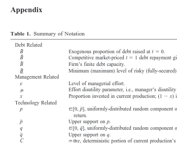
Table 1. Summary of Notation
Debt Related
B Exogenous proportion of debt raised at t50.
Bˆ Competitive market-priced t51 debt repayment given B.
B# Firm’s finite debt capacity.
B Minimum (maximum) level of risky (fully-secured) debt. Management Related
e Level of managerial effort.
m Effort disutility parameter, i.e., manager’s disutility isme2.
x Proportion invested in current production; (12x) invested in intangible assets.
Technology Related
p [[0, p#], uniformly-distributed random component of current production’s return.
p# Upper support on p.
q [[0, q#], uniformly-distributed random component of intangible’s return.
q# Upper support on q.
C [uxe, deterministic portion of current production’s return. D [f(12x)e, deterministic portion of intangible’s return.
u Positive scale parameter in C.
f Positive scale parameter in D.
d [[0, 1], proportion of current production’s t52 return realized in a t51 liquidation.
D [dzE(pC), current production’s t51 salvage value (intangibles have zero
salvage). Miscellaneous
p1 [Bˆ /C, lowest realization of p for which the firm continues as a going concern.
p2 [(Bˆ2 D)/C, lowest realization of p for which the firm is solvent only after
Proof of Proposition 2.
Writing equation (5) as the implicit function, J50, and then totally differentiating yields:
dBˆ dz 52
Jeez1Jz JBˆ1JeeBˆ
, z[$p#, q#,u,f,d,m, x%,
and
dBˆ dB5
2JB JBˆ1JeeBˆ
.
Noting that JB5 21, footnote 11 implies that sgn(dBˆ /dz)5 2sgn( Jeez1Jz). Taking the indicated derivatives completes the proof for part (a). The sign of dBˆ /dx is ambiguous; after tedious algebra, and using equation (3) to simplify the expression, we have:
Jeex1Jx5
F
~Bˆ22D2!e
2x~2mp#uxe32Bˆ2!
GS
4me2 q#f2
D
; (A1)and noting, from footnote 9, that [z].0 completes the general statement in part (b). To show the specific claim, define ec[q#f/8m. Then, from equation (A1), dBˆ /dx:0 if and only if e*"ec, at a given debt level. For B[[0, B], an increase in Bˆ implies x increases (this is formally shown in Proposition 5 below) and so, from Proposition 4, e* is monotonically decreasing and, using equation (A9), e*uB5B . ec; hence, e*(B) . ec, @B[[0, B]. Additionally, it can be shown that e*(B#) , ec. Consequently, by continuity, part (b) follows.
First Order Condition for the (risky debt) Investment Problem.
Differentiating equation (6) with respect to x, and simplifying yields:Vx5
S
p#u 2 q#f2
D
~e1xex!1 q#f2
S
Bˆp#ux21ex
D
1HF
p#ux1 q#f2 ~12x!
G
eBˆ212
F
~12d!1q#f~12x!p#ux
GJ
dBˆdx, where
e1xex52 1 Hee
S
4me2q#f
2
D
. (A2)As from equations (A1) and (A2), sgn(dBˆ /dx)5 2sgn(e1 xex), it follows that the first order condition, Vx50, can be satisfied regardless of the sign of ex.
Derivation of the Maximum Debt Capacity, B
#
.
As indicated in Section IV,
and
Bˆ~B#!5~11d/ 2!p#C. (A4)
Substitution of equation (A4) into equation (3), and then into equation (6) yields:
e#5 1
where from footnote 10, effort e# is defined ase# 5 infe*[51e* and, therefore, equation
(A3) identifies the limiting amount of priceable debt.
Proof of Proposition 3.
Totally differentiating the first order condition, Vx 5 0, associated with equation (6), yields:
Noting that the denominator of dx*/dBˆ is the second order condition for the investment problem, which from footnote 14 is negative, and using dBˆ /dB . 0, we have that sgn(dx*/dB) 5 sgn(VxBˆ 1 VxeeBˆ), where the first (second) term is the direct (indirect) effect of Bˆ on x*. Taking the indicated partial derivatives yields:
VxBˆ5
F
p#ux1Derivation of the Maximum Fully-Secured Debt Level, B.
As indicated in the first subsection of Section V, B is given by:B;dE@p#C~x, e!5d
Using equations (8) and (A7), the first order condition for optimal investment yields:
x*5x*uB5B5
2dq#f
4~2p#u 2q#f!. (A8)
We note that equation (A8) is well-defined, i.e., x*[(0, 1), if and only if:
2p#u ,q#f
S
12d 4D
;otherwise, the investment constraint is binding, i.e., x*51. Further, there are two other solutions to the first order condition evaluated at B. The first, x5 q#f/(q#f22p#u).1, is rejected as infeasible; the second, x5 0, is rejected as it implies B 5 0, i.e., that fully-secured debt is not possible. Additionally, substituting equation (A8) into equation (8) provides the following expression for optimal effort:
e*5e*uB5B5 q#f 4m
S
12d
4
D
. (A9)Finally, substituting equations (A8) and (A9) into equation (A7) gives:
B52p#u~dq#f!
2~12d/4!
32m~2p#u 2q#f! .
Proof of Proposition 4.
Follows from taking the indicated partial derivatives of equation (8).
Proof of Proposition 5.
Using equation (6), the first order condition to the investment problem can be written as:
Vx;x3 1 ax21bB50, (A10)
wherea;q#f/~2p#u 2q#f!,0 andb;@2m/p#u~2p#u 2 q#f!#a .0. Totally differentiating equation (A10) yields:
dx* dB 52
VxB Vxx
5 2b
3x212ax.0,
where the inequality follows from the assumption that the second order condition holds, i.e., that Vxx, 0. In a similar manner, it can be verified that d2x*/dB2,0.
References
Bradley, M., Jarrell, G., and Kim, E. H. 1984. On the existence of an optimal capital structure: Theory and evidence. Journal of Finance 39:857–878.
Caravatti, M.-L., Sept./Oct. 1992. Why the United States must do more process R&D.
Research-Technology Management: 8–9.
Chan, S. H., Martin, J., and Kensinger, J. 1990. Corporate research and development expenditures and share value. Journal of Financial Economics 26:255–276.
Chauvin, K., and Hirschey, M. 1993. Advertising, R&D expenditures and the market value of the firm. Financial Management 22(4):128–140.
Doukas, J., and Switzer, L. 1992. The stock market’s valuation of R&D spending and market concentration. Journal of Economics and Business 44:95–114.
Grossman, S., and Hart, O. D. 1982. Corporate financial structure and managerial incentives. In The
Economics of Information and Uncertainty (J. J. McCall, ed.). Chicago: University of Chicago
Press, pp.
Harris, M., and Raviv, A. 1990. Capital structure and the informational role of debt. Journal of
Finance 45:321–349.
Jensen, M. C. 1986. Agency costs of free cash flow, corporate finance, and takeovers. American
Economic Review 76:323–329.
Jensen, M., and Meckling, W. 1976. Theory of the firm: Managerial behavior, agency costs, and capital structure. Journal of Financial Economics 3:305–360.
Long, M., and Malitz, I. 1983. Investment patterns and financial leverage. National Bureau of
Economic Research.
Myers, S. C. 1977. Determinants of corporate borrowing. Journal of Financial Economics 5:146– 175.
Myers, S. C. 1984. The search for optimal capital structure. Midland Corporate Finance Journal 1:6–16.
Quirmbach, H. C. 1993. R&D: Competition, risk, and performance. Rand Journal of Economics 24:157–197.
Rosen, R. J. 1991. Research and development with asymmetric firm sizes. Rand Journal of
Economics 22:411–429.
Smith, C. W., Jr., and Warner, J. B. 1979. On financial contracting: An analysis of bond covenants.
Journal of Financial Economics 7:117–161.
Smith, C. W., Jr., and Watts, R. L. 1992. The investment opportunity set and corporate financing, dividend, and compensation policies. Journal of Financial Economics 32:263–292.
Solt, M. E. 1993. SWORD financing of innovation in the biotechnology industry. Financial
Management 22:173–187.
Stulz, R. M. 1990. Managerial discretion and optimal financing policies. Journal of Financial
Economics 26:3–27.
Stulz, R. M., and Johnson, H. 1985. An analysis of secured debt. Journal of Financial Economics 14:501–521.
Zantout, Z. Z. 1997. A test of the debt monitoring hypothesis: The case of corporate R&D expenditures. Financial Review 32:21–48.