*Corresponding author. Tel.:#00-31-40-247-2869. E-mail address: [email protected] (K. van Don-selaar).
The impact of material coordination concepts on planning
stability in supply chains
K. van Donselaar
*
, J. van den Nieuwenhof, J. Visschers
Faculteit Technologie Management, Eindhoven University of Technology, Vakgroep IDL, P.O. Box 513, 5600 MB Eindhoven, The Netherlands Received 31 March 1998; accepted 1 March 2000
Abstract
The goods#ows in supply chains can be managed based on either the purchase orders of the next company in the chain or on the demand information from the end customer in the total supply chain. Many standard software packages which are meant for controlling goods#ows are based on the purchase orders of their immediate customers (in accordance with the MRP logic). In this paper it is investigated how the type of demand information used in#uences the stability of the planning in the supply chain. For this purpose a simulation experiment was set up, using data from a truck manufacturer in the Netherlands. This company was confronted with the choice to either stick to its own planning logic (based on undistorted demand information from the end of the supply chain) or to change over to a standard package based on the MRP-logic. This experiment reveals how instable the planning in a supply chain may become if the wrong demand information is being used. The experiment also shows which factors in the production environment as well as in the market place have the biggest impact on the instability of the planning. The results were discussed with the development department of a major software company. Based on the results the software company is now considering to adapt the planning logic in their standard software package. ( 2000 Elsevier Science B.V. All rights reserved.
Keywords: Supply chain management; Material coordination; Order release
1. Introduction
DAF Trucks, a truck manufacturer in The Neth-erlands, assembles to order. Eight years ago they had to decide how to control their raw materials and (sub)components. They decided not to use MRP to control their good#ows. Instead they used an algorithm for the calculation of material requirements, which is based on LRP (see Ref. [1]). The essence of LRP is the fact that demand in-formation from the "nal customer is transferred
directly to each of the stages in the supply chain. In MRP, the demand from the"nal customer is "rst turned into planned orders for the"nal production stage. These planned orders are then exploded to the next stage in the supply chain, etc. So in the MRP-logic the demand information from the"nal customer is distorted before it is exploded. The transparancy of the supply chain, obtained by using undistorted demand information from the"nal cus-tomer, was one of the main reasons for DAF to choose for the LRP-logic. Recently, however, DAF Trucks has decided to change from this house-made application to a standard Enterprice Resource Planning package. Since all large stan-dard ERP-packages are based on the MRP-logic,
DAF and the ERP-software supplier were con-fronted with the following dillemma: either to give up the close link with the"nal customer's demand or to adapt the standard software.
In order to make this decision, DAF Trucks and Eindhoven University started a research project. The aim of this project was:
(1) to determine the added value of the direct link with the"nal customer's demand,
(2) to "nd out which product-, production- or market-characteristics have the biggest impact on the stability of the planning.
Hereto interviews were carried out with the plan-ners and the suppliers who used the results from the LRP-planning logic. These interviews were used to set up a simulation experiment. This simulation experiment revealed that in the DAF-situation the planning of components was more stable when there was a direct link with the "nal customer's demand. This"nding was also con"rmed by DAF's suppliers; they noticed that DAF's material requirements were very stable over time compared to the requirements of DAF's competitors. This stability reduces the need for expensive emergency orders.
The results of this research project are reported in this paper. In Section 2 the literature is reviewed. In Section 3 the LRP and MRP-planning logic are described brie#y. In Section 4 the simulation experiment is explained. The results are presented in Section 5. These results have also been presented to one of the world's leading standard ERP-pack-age suppliers. Based on these results, and recognis-ing the fact that supply chains who are the best in information exchange and control of goods#ows, may have the best competitive position, the soft-ware supplier is considering to adapt the planning logic in its standard ERP-package.
2. Literature review
In the last two decades there have been a number of researchers who have recognised the importance of planning nervousness in MRP systems. For example, Kadipasaoglu and Sridharan [2] state `Schedule nervousness caused by uncertainty in demand or supply or by dynamic lot-sizing can be
an obstacle to e!ective execution of material requirements planning systemsa. A number of strat-egies are proposed to deal with this nervousness. Blackburn et al. [1] propose the following ranking of strategies to dampen nervousness in MRP sys-tems (for the explanation of each of these strategies we refer to their article [3]):
(1) change cost procedure;
(2) forecast beyond planning horizon;
(3) freezing the schedule within the planning hor-izon;
(4) lot-for-lot; (5) bu!er stock.
Ho [4] adds two more strategies. His strategies are based on the distinction between large and small changes.
As Kadipasaoglu and Sridharan [2] point out, allmost all literature on planning nervousness is restricted to only one level (the end-item level) or assumes that the environment is deterministic. Examples are the papers of Kropp et al. [5,6], Carlson [7], Blackburn et al. [3], Jensen [8], Inder-furth [9], De Kok et al. [10] and Heisig [11]. The paper of Kadipasaoglu and Sridharan [2] together with the papers of Ho [4] and Zhao and Lee [12] are exceptions to this.
Still, all the above literature on planning ner-vousness in multi-echelon systems assumes that the MRP-logic should be used. This is probably due to the fact that all standard ERP software packages are based on MRP. In this paper we address the question to what extend the planning nervousness can be diminished by using an alternative planning logic. In e!ect, we try to demonstrate that the true cause of all nervousness is the MRP planning logic itself.
Furthermore we will also investigate the impact of several parameters (like the demand uncertainty, the lot-sizes and the product structure) on the nervousness.
3. The MRP- and LRP-logic
Example
Component C Raw material RM
safety stock"20; on hand"30; leadtime"1 week; lot-size "4 weeks.
safety stock"10; on hand"11; leadtime"2 weeks; lot-size"4 weeks.
Week 0 1 2 3 4 5 6 7 !1 0 1 2 3 4 5 6 7
Gross requirements 10 10 10 10 10 10 10 10 10 10 10 10 10 10
Sched. receipts 40
Available balance 10 0 !10 !20 !30 !40 !50 !60 111 1 31 21 11 1 !9 !19
Pl. order due 40 20 19
Pl. order release 40 20 19
1The total inventory in the chain is 30 (C)#11 (RM)"41. and the total safety stock in the chain is 20 (C)#10 (RM)"30, so the available balance in the chain is 41}30"11 units RM. Donselaar [1]. Basically, LRP is a time-phased
echelon stock control policy as introduced by Clark and Scarf [14].
Let's"rst assume alinearproduct structure: one component C is made from one raw material RM. The time-phased gross requirements for C are assumed to be the input for both LRP and MRP. MRP turns these gross requirements into plan-ned orders for C, by taking into account the inven-tory, the scheduled receipts, the safety stock, the lot-size and the leadtime of C. These planned orders are then assumed to be the gross requirements for raw material RM. For raw material RM these gross requirements are turned into planned orders by using the same logic as applied for the component C.
LRP calculates the planned orders for C in the same way as MRP. The planned orders for RM, however, are derived directly from the gross requirements of C. For this purpose the gross requirements of C are o!-setted with the leadtime
of C and then exploded to RM. Note that no netting and no lot-sizing is involved here! These numbers constitute the gross requirements of RM. At the same time the inventory plus the scheduled receipts of C are summed up and exploded to RM. This downstream-inventory-position is raised with the local inventory of RM. This results in the total inventory in the supply chain. Now the gross re-quirements of RM are netted with this &supply
chain inventory'. (In case there are safety stocks, these safety stocks are also exploded separately and subtracted from the supply chain inventory before the netting takes place.) Next these net require-ments are turned into planned orders for RM by taking into account the scheduled receipts of RM, the lot-size and the leadtime of RM, just like in the MRP-logic.
Below an example is given to illustrate how LRP works. In this example it is assumed that the lot-size for C and RM is equal to&4 weeks of net requirements'. This type of lot-sizing rule is very common at DAF Trucks as well as at many other companies. The advantage of such a lot-size rule compared to a"xed number of products (like&the lot-size is 40 products') is that this rule automati-cally adapts the lot-size when the average demand changes. A second bene"t is that this lot-size rule "ts better in environments with "xed production cycles, that is: environments where it is possible to produce a product only once everyx weeks.
In environments with divergent product
Table 1
position of the component separately. At the raw material level the inventory position of all compo-nents with the same raw material is added up before the gross requirements of the raw material are netted with this total inventory. As a result the LRP logic assumes inventories are always balanced and therefore sometimes LRP may determine that no planned order for RM is needed, while one of the components is short of inventory.
When LRP was implemented at DAF Trucks, the planners of DAF insisted that these planning errors would not occur. To prevent this, an adapta-tion of the pure LRP-logic was implemented: Before exploding the gross requirements of the components to RM, the gross requirements of each component were netted "rst with the inven-tory of this component. Basically this leads to an explosion logic which is equal to&LRP with netting' or &MRP without lot-sizing'. At DAF &LRP with netting' is applied both for linear and divergent structures.
4. The simulation experiment
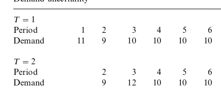
In the simulation experiment, linear as well as divergent product structures were simulated. In the linear product structures a component C was made from one raw material RM. In the divergent case, two components, C1 and C2, were made from raw material RM. Demand for the components is known for the"rst two periods and is uncertain for the remaining periods. The aim of the simulation was to determine the performance of MRP and LRP (in its pure form) measured by the service level, the inventory levels and the planning ner-vousness.
For the component, requirements for the "rst two periods were known customer orders. To simu-late demand uncertainty, the true demand in the second planning period at¹#1 deviates from the expected demand leveldin the third planning peri-od at ¹ by using an uniform distribution with averaged. The average is set at 10 units. The inter-val of the uniform distribution is formed by a user de"nable variable, which must be entered at the beginning of the simulation. Table 1 shows an example of the above.
The leadtime of all products is assumed to be 2 periods. Finite capacity restrictions are not taken into account explicitly. Planned orders are recal-culated every period, whereas scheduled receipts are considered to be&"rm', they cannot be delayed or rushed. Furthermore the model has a build-in material check at the release moment of the pro-duction order of C. If the inventory level of raw material RM is insu$cient to meet the require-ments of the production order of C, then the order amount of C is set equal to the inventory level of RM. This holds for linear product structures. In case of divergent product structures, if there is a shortage of RM, the scarce raw materials RM are allocated to C1 and C2 in such a way that the inventory of each of these products is equal (since the products in our simulation have demand distri-butions with the same mean and variance). Even if there is no enough inventory to do this, the inven-tory is given to the product with the least inveninven-tory. Finally, the (planned) orders for RM are always rounded o!to a multiple of 10 units. This repres-ents the fact that suppliers only want to deliver in minimal packing quantities.
The performance of both planning systems is measured by the following output-parameters:
(1) Service level:
the average probability of stock-out during a replenishment cycle. (2) Inventory
level:
average total amount of inventory of product C and raw material
RM. (3) Planning
nervousness:
2This order has now become a scheduled receipt and is therefore no longer a planned order
3&variability in demand'is de"ned here as the deviation be-tween maximum and average demand in terms of a percentage of the average demand.
To illustrate the planning nervousness, consider the following example: still a planned order in the next planning run (although the order quantity may be di!erent!)? If not, we increase the number of reschedules with 1.
f If there was no planned order in¹#x, is there still none in the next planning run (at period ¹#1)? If there is one, we increase the number of reschedules with 1.
So in the example above the number of reschedules is 1. Note that our de"nition of planning ner-vousness focusses on changes in timing rather than on changes in the quantity of the planned order. This is due to the fact that DAF and its suppliers want to minimise disruptions in the production sequence, since this would imply extra set-up time. So our measurement of nervousness focusses on &setup-oriented planning instability' as de"ned by Heisig [11]. For appropriate de"nitions of& quanti-ty-oriented planning instablity', i.e. planning ner-vousness in situatiuons in which changes in the order quantity are most disruptive, we refer to De Kok and Inderfurth [10].
Finally, note that the nervousness of the planned orders is also an indicator for the number of re-scheduling messages which will be generated for the scheduled receipts.
The outcomes of the values of these performance measurements are based upon 500 simulation runs. Each simulation run simulates the planning during
30 consecutive periods. The"rst 10 simulation peri-ods are used for initialisation. The last 20 periperi-ods of each simulation are used for the measurements of the output-parameters. So for every scenario (i.e. a combination of input-parameters) 10.000 periods were simulated. Every period in the simulation a planning is made for the raw materials and the components with a planning horizon equal to 17 periods (which is longer than the cumulative lead-time plus the largest lot-size). This planning hor-izon is equal for all scenarios.
The following input parameters were varied:
(1) the lot-size for the component(s):
2, 4 or 8 periods of net requirements
(2) the lot-size for the raw material: (4) product structure: linear or divergent
Since the lot-size of the raw material was always chosen larger or equal to the lot-size of the com-ponent(s), in total 24 simulation experiments were carried out.
5. Results
In the simulation experiments the safety stock norms for MRP and LRP were chosen equal. On average the simulations with MRP resulted in a slightly higher service level (93.1% for MRP ver-sus 91.5% for LRP), but in considerable more inventory on hand (67.3 units for MRP versus 54.9 units for LRP).
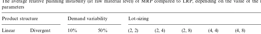
Table 2
The average relative planning instability (at raw material level) of MRP compared to LRP, depending on the value of the input-parameters
Product structure Demand variability Lot-sizing
Linear Divergent 10% 50% (2, 2) (2, 4) (2, 8) (4, 4) (4, 8) (8, 8)
2.7 6.5 6.9 2.3 7.9 4.8 4.5 3.7 3.4 3.5
Thanks to this additional inventory, MRP is better able to meet the planned orders of the components and therefore, the planning of these components is more stable.
Since LRP does not focus on exact lot-sizing quantities (see the gross requirements for RM in the example we used to illustrate LRP), LRP regularly will be short of one or two raw materials. Suppose, for example, that the next order to be released for the component C equals 40 units, while at that moment the inventory level of the raw material is only 39 units. Then LRP will release 39 in stead of 40 units of C. This may imply that the next planned order for C will be planned one period earlier in the next planning run. This is the instability of the planning of the component(s). In our simulations we found that the instability at component level decreases rapidly by simply adding a small amount of inventory to the raw material RM. By raising the inventory in the LRP simulation to the level of inventory we obtained in the MRP simulations (by raising the safety stock norm for the raw material in the LRP calculation), we noticed that both the service levels and the planning stability at the component level of the MRP and LRP controlled systems were approximately equal.
It may also be argued that the instability at the component level for LRP is no problem at all, since the old planned orders at the component level are not used at all by LRP. So the fact that the ultimate orders deviate from the planned orders is harmless for strictly linear and divergent structures.
According to the simulation results, the only true di!erence between the LRP and MRP planning is the relatively high instability of the MRP planning at the raw material level. As a measure for this we used the ratio of&number of reschedules for MRP' over&the number of reschedules for LRP'.
Table 2 shows the average of this ratio for all simulation experiments per input variable. For example, the 6.5 is the average ratio over all 12 experiments in which we used a divergent product structure. For detailed simulation results we refer to the appendix.
The results in Table 2 show that all three input parameters can have a strong impact on the plann-ing nervousness of MRP. The maximum ratio was 17.8. This ratio holds for a divergent system with low demand variability and small lot-sizes. For this system apparently MRP is approximately 17 times more nervous compared to LRP. On average MRP was 4}5 times more nervous than LRP (with both systems having the same inventories and service levels). Even in the best case, MRP was still 30% more nervous than LRP.
For a good interpretation of these results, it should be mentioned that in the cases where MRP is relatively very nervous compared to LRP, the
absolutenumber of replanned orders is also large. If we look at the absolute number of replanned orders (see the Appendix), we notice the number of replan-ned orders goes up if demand uncertainty increases (similar with the "ndings of Heisig [11], who studied nervousness in 1-echelon systems) or if the lot-sizes decrease.
It should be stressed here that our results are very dependent on the dynamic lot-sizing rule ap-plied in the planning. On the other hand, it has been explained why this lot-sizing rule is often applied in practice.
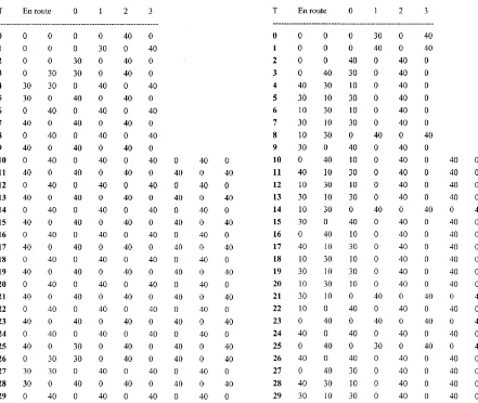
Fig. 1. The planning for 30 consecutive periods with MRP resp. LRP for a divergent system with all lot-sizes equal to 2 weeks net requirements.
the planning is stable, we see straight diagonals with every order being equal to the same number of units (in this case 40 units).
Another way of recognising the (in)stability is by looking only at the "rst column. This shows the pattern of the scheduled receipts in consecutive periods. For MRP this is (from period 10 on):
0, 40, 10, 30, 10, 30, 10, 30, 0, 40, 30, 10,
whereas for LRP this is:
0, 40, 0, 40, 0, 40, 0, 40, 0, 40, 0, 40.
6. Conclusions
without taking into account the lot-sizing. We saw that three variables all have a strong impact on this potential nervousness of MRP: the lot-sizes, the demand uncertainty and the product structure. In the worst case (i.e. small lot-sizes, low demand uncertainty and a divergent product structure) the MRP-planning was 17 times more nervous than its alternative, called LRP. On average MRP was 4}5 times more nervous than LRP.
These results have been discussed with a major supplier of a standard ERP-software package. Based on the results of these simulations and on the positive experience of a manufacturer and his sup-pliers, who have been using the alternative for MRP already for some years, this software supplier is considering to adapt the planning logic in his standard package.
Appendix A. Detailed simulation results
Lot-Linear Divergent Linear Divergent
(2, 2) 12.1 16.0 16.7 19.2
The number of replanned orders at raw material level in caseMRPis applied. This number is given
for several scenarios (with di!erences in lot-sizing, demand variability and the product structure).
Lot-Linear Divergent Linear Divergent
(2, 2) 1.9 0.9 6.6 4.0
The number of replanned orders at raw material level in case¸RPis applied. This number is given
for several scenarios (with di!erences in lot-sizing, demand variability and the product structure).
References
[1] K. van Donselaar, The use of MRP and LRP in a stochas-tic environment, Production Planning and Control 3 (3) (1992) 239}246.
[2] S.N. Kadipasaoglu, V. Sridharan, Alternative approaches for reducing schedule instability in multi-stage manufac-turing under demand uncertainty, Journal of Operations Mangement 13 (1995) 193}211.
[3] J.D. Blackburn, H.D. Kropp, R.A. Millen, A comparison of strategies to dampen nervousness in MRP systems, Management Science 32 (4) (1986) 413}429.
[4] C. Ho, Evaluating the impact of operating environments on MRP system nervousness, International Journal of Production Research 27 (1989) 1115}1135.
[5] D.H. Kropp, R.C. Carlson, J.V. Jucker, Use of dynamic lot-sizing to avoid nervousness in material requirements planning systems, Journal of Production and Inventory Management 20 (1979) 40}58.
[6] D.H. Kropp, R.C. Carlson, J.V. Jucker, Heuristic lot-sizing approaches for dealing with MRP system nervousness, Decision Sciences 14 (2) (1983) 156}169.
[7] R.C. Carlson, S.L. Beckman, D.H. Kropp, The e! ec-tiveness of extending the horizon in rolling production schedules, Decision Sciences 13 (1) (1982) 129}146. [8] T. Jensen, Measuring and improving planning stability of
reorder point lot-sizing policies, International Journal of Production Economics 30}31 (1993) 167}178.
[9] K. Inderfurth, Nervousness in inventory control: Analyti-cal results, OR Spektrum 16 (1994) 113}123.
[10] A.G. De Kok, K. Inderfurth, Nervousness in inventory management: comparison of basic control rules, European Journal of Operational Research 103 (1997) 55}82. [11] G. Heisig, Planning stability under (s, S) inventory control
rules, OR Spektrum 20 (4) (1998) 215}228.
[12] X. Zhao, T.S. Lee, Freezing the master production sched-ule for material requirements planning systems under de-mand uncertainty, Journal of Operations Management 11 (2) (1993) 185}205.
[13] J. Orlicky, Material Requirements Planning, McGraw-Hill, London, 1975.