*Corresponding author.
E-mail address:[email protected] (E. Luciano).
Cycles optimization: The equivalent annuity and the NPV
approaches
Elisa Luciano!,
*, Lorenzo Peccati"
!Dipartimento di Statistica e Matematica Applicata, University of Turin, Piazza Arbarello 8, I-10121 Turin, Italy
"Istituto di Metodi Quantitativi, Universita` **Luigi Bocconi++, via Sarfatti, 25, I-20136 Milan, Italy Received 20 April 1998; accepted 23 December 1999
Abstract
The paper discusses the use of a generalized version of the equivalent annuity principle, which takes into account interest rate#uctuations over time. When dealing with applications over a sequence of cycles, e.g. plant replacement ones, the equivalent annuity is usually de"ned with reference to each single cycle or to the whole sequence. First, we study the correspondence between net present values and equivalent annuities as de"ned above in optimization problems. We show that only the second de"nition is appropriate for optimization, whenever the length of the cycle is a choice variable. However, also the second is not necessarily correct, when the horizon is "nite. Then, we discuss the corresponding problems of optimality, both with an in"nite and a"nite sequence of cycles. Applications to a simple plant replacement problem are illustrated: they show how di!erent the optimal decisions can be from the equivalent annuity ones. ( 2001 Elsevier Science B.V. All rights reserved.
Keywords: Net present value; Equivalent annuity; Plant renewal
1. Introduction
Many problems in Production Economics turn out to consist of the"nancial evaluation of a"nite or
in"nitechainof cash#owcycles. The"nancial evaluation generally consists in computing the net present
value of the cash #ows of the whole chain. However, another approach}the equivalent annuity one}is sometimes introduced. The equivalent annuity is the constant cash#ow intensity which has the same present value of the original in#ow and out#ow stream. Due to the character of the de"nition itself, it is generally argued that using the net present value or its equivalent annuity is the same.
This paper aims to show the possible error in this statement, for optimization purposes. In detail, we are reminded that the equivalent annuity can be de"ned either cycle by cycle or for the whole chain. We show the lack of correspondence between net present value and equivalent annuity when the length of the cycles is
a choice variable and either the horizon (i.e., the number of cycles) is"nite, or the cycle by cycle annuity is considered.
The argument is relevant for practical purposes, since decisions taken with the two approaches can di!er signi"cantly. We show this with reference to a plant replacement problem: via equivalent annuity we are led to strategies which are not the same as the net present value ones and have a signi"cantly smaller value today. In the numerical examples, the di!erences between the values produced by the two policies range from 10% or 14% to more than 100%: in one of our illustrative cases, the equivalent annuity leads to a negative value for the replacement plan, while via net present value we have positive worth.
The consequence of our argument is that the equivalent annuity is useful in order to represent a given cash
#ow stream; it is not for optimization purposes in general. In the latter case, on the contrary, it can produce suboptimal decisions.
In the previous literature, as far as we know, the limits of application of the equivalent annuity principle were not known, as the corresponding cases had not been studied.
The objectives of the paper are as follows. In Section 2 we describe the usual equivalent annuity setup, with constant interest rates, and put into evidence on the one side the correspondence between maximizing (or minimizing) net present values and annuities over the whole chain, on the other the lack of correspondence between maximizing present values and equivalent annuities over a single cycle.
In Section 3 we analyze the problem in a general framework, corresponding to variable interest rates. As for the in"nite horizon case, the results obtained in the constant rate case still hold. As for the"nite horizon one, the correspondence over the whole chain breaks down. In Section 4 we illustrate the previous correspondence arguments with reference to a simple plant replacement problem. In Section 5 we study the optimization technique for the in"nite horizon case. In Section 6 we do the same for the"nite horizon one. Section 7 applies the techniques of Section 6 to the plant replacement example. Section 8 concludes and outlines further applied research.
2. Standard setup
Let us consider the case of plant replacements or of inventory management, as presented in Thorstenson [1] or Babusiaux [2], under the usual assumption of constant interest rates. We are given:
f a sequence of increasing maturitiest
0,t1,t2,2,
t
0"0;t1"z1;t2"z1#z2;2; tn" n + s/1
z
s;2,
which de"nes achainof consecutivecycleswith respective lengthsz
s'0,s"1, 2,2;
f the sequence of the corresponding discounted or net present values (from now on NPVs)G
s, computed at the beginning of the cycle (t
s~1). To be more precise, let us assume that thesth cycle, which starts at time t
s~1, requires a discrete cash out#ow of amount Is and provides continuous cash in#ows with intensityo
s(t) att3(ts~1,ts) and a"nal payo!Js. In this case the NPV for thesth cycle, computed att
s~1, is
G
s"!Is#
P
tsts~1 o
s(t)e~d(t~ts~1)dt#Jse~d(ts~ts~1), s"1, 2,2,
1A special case which is frequently encountered in the applications is that of lattice maturitiest
s"sq, withq'0, and identicalGs,g.
In such a situation the NPV of the whole chain,G, is given byG"g/(1!e~Lq)
2The key argument for the former result is easily focused. Reconsider Eq. (2.2) and suppose that you are maximizingG
sthrough the choice of some variables, one of which isz
sitself. Suppose thatGsis di!erentiable. The"rst order necessary condition requires that at interior (positive) maxima
LG
s/Lzs"0
holds, while the corresponding condition onC
s"Gsa(zs,d) requires
LG
s
Lz
s
a(z
s,d)#Gs
La(z
s,d)
Lz
s
"0. The two conditions coincide i!G
s"0. A simple consequence is thatmaximizing(or minimizing) Gs,in general,is not the same as
maximizing(or minimizing)C
s.
The NPV of the whole chain is then
G"`+=
s/1
e~dts~1G
s (2.1)
provided that the series converges, as usually occurs in the models having practical interest.1 In order to obtain a quantity with a more natural interpretation thanG
s orG, it is sometimes suggested (see, for instance, the works of GrubbstroKm and Thorstenson [3] or GrubbstroKm and Thorstenson [4]) to compute theequivalent annuityof a given cash#ow. The equivalent annuity is the continuous and constant cash#ow intensity which is"nancially equivalent to the NPV.
In principle there are two possibilities:
1. to determine the equivalent annuityC
s for thesth cycle, with NPVGs, through the equation
P
zs 0C
se~dtdt"GsNCs"Gsa(zs,d), s"1, 2,2, (2.2)
wherea(z, d)"$ d/(1!e~dz) is the continuous repayment instalment due in order to extinguish a unitary debt in zyears with force of interestd, usually denoted with the actuarial notationa6
z6@(d);
2. to determine the equivalent annuityCfor the whole sequence of cycles with NPVGthrough the equation
P
`= 0Ce~dtdt"GNC"Gd. (2.3)
The two possibilities have di!erent consequences when dealing with optimization problems, for the following reason. The NPVsGandG
s are generally a function of several variables, within which there may be some elements of the maturity sequenceMt
sN: in most applications then we are asked to maximize or minimizeGor
G
sAs concernsthrough a correct choice of the underlying variables, in particular of (some or all) the cycle lengthsC, Eqs. (2.2) and (2.3) show that C is proportional to the NPVs, so that maximizingMz(orsN. minimizing)Gandmaximizing(or minimizing)Cis the same, as already noted by GrubbstroKm and Thorsten-son [3] and ThorstenThorsten-son [1].
f As concerns theC
s, on the opposite side, the two strategies:maximizing(or minimizing)Gs and
f maximizing(or minimizing)C
s are not the same, since2C
This paper is di!erent from previously published works in that it considers a more general context, of variable interest rates. It studies the equivalent annuity and the corresponding optimization problems both for the"nite and the in"nite horizon (or number of cycles) case. It analyzes the optimization problems both in general and by using as an example a plant replacement case.
3. A general framework
Let us set up a general framework, within which we shall study the problem.
First of all, let us suppose that interest rates are variable over time: formally, that the discounting ratedis a function of time,d"d(t). The discount factor e~dtwill be replaced with exp(!:t
0d(u) du). Throughout this paper we shall always assume that d(t) is continuous and positive: the "rst assumption guarantees that discount factors are well de"ned for"nitet, the second}which is natural in nominal terms}makes them decreasing over time. Also, we will assume that lim
t?`=exp(!:t0d(u) du)"0: the discount factor is not only decreasing, but also in"nitesimal as time increases.
In general, the present value atx of 1$available aty*xwill be
U(y,x)"exp
A
!P
yx
d(u) du
B
.For the sake of simplicity, we shall write/(y) forU(y, 0):
/(y)"$ U(y, 0)"exp
A
!P
y0
d(u) du
B
. (3.1)We call Generalized Net Present Value (GNPV) a NPV computed with these discount factors.
Secondly, we should keep in mind that the (G)NPV implicitly assumes that investments are"nanced with equity only. In general a mixed capital structure can be expected: therefore we need an extension of the NPV, in order to cope with these problems. We shall use the framework introduced in the works of Peccati [5], GrubbstroKm and Ashcroft [6], Gallo and Peccati [7] and, recently, with reference to inventory problems, in Luciano and Peccati [8,9]. From a practical viewpoint the extension consists in replacing the standard (G)NPV with the algebraic sum of the (G)NPVs of investments and"nancing operations. As a consequence, in the sequel the term (G)NPV refers to this algebraic sum.
Sincednow is a function of time, the (G)NPV for thesth cycle, computed at t
s~1, is
G
s"!Is#
P
tsts~1 o
s(t)U(t,ts~1) dt#JsU(ts,ts~1), s"1, 2,2. (3.2)
With an in"nite number of cycles, Eq. (2.1) provides us with the global result of the whole chain and becomes
G"`+=
s/1 G
s/(ts~1) (3.3)
whereG
s is given by Eq. (3.2). We shall assume in what follows that the above mentioned series converges. Also, in order to de"ne equivalent annuities, we assume that:`0=/(t) dt(R.
With reference to the new meaning ofG
s and to the equivalent annuity, the presence of a time-varying interest intensity implies that
1. the equivalent annuity for one cycle must satisfy the equation
P
tsts~1 C
3We thank an anonymous referee for having pointed out the a fortiori argument. However, a formal proof can be found in Appendix A.
whence
C
s"
G
s :ts
ts~1U(u,ts~1) du
; (3.4)
2. the equivalent annuity for the whole chain must satisfy the equation
P
`= 0C/(t) dt"G
so that it is
C" G
:`0=/(t) dt. (3.5)
The non-correspondence between maximizing (or minimizing) C
s and maximizing (or minimizing)
G
s through an appropriate choice of the lengthzs, which we illustrated in the introduction fordconstant, a fortioriholds true fordnon-constant.3
On the other hand, it is easy to show that maximizing (or minimizing) G, the in"nite sequence NPV, described in Eq. (3.3), is the same as maximizing (or minimizing) the equivalent annuity for the whole sequence,C. The non-correspondence between optimizingC
sandGson the one side and the correspondence between optimizingCcon"rms the correspondence/disagreement results obtained under constantd.
However, with non-constantdwe also want to analyze what happens with a"nite number of cycles, i.e. with a"nite horizon:G
n`1"Gn`2"Gn`3"2"0 in Eq. (3.3). The global result of the "nite chain of cycles, which we denote withGM
n, is
GM
n" n + s/1
G
s/(ts~1). (3.6)
Having excluded the usefullness, for optimization purposes, of using the equivalent annuity over single cycles, we de"ne for this"nite horizon case only the equivalent annuity for the whole chain. We denote it withCMn. SinceCM n must be such that
P
tn 0CM n/(t) dt"GMn
we have
CMn"GMn/
P
tn 0/(t) dt. (3.7)
It follows from the de"nition ofCMnitself and it is demonstrated in Appendix A thatmaximizing(or minimizing)
GMn through an appropriate choice of the lengthz
s is not the same as maximizing(or minimizing)the present
value of CMn: in the "nite horizon case then optimizing with respect to the NPV or with respect to the equivalent annuity gives di!erent results, even if we take into consideration the whole sequence of cycles.
Table 1
Summary of correspondence results
Horizon Interest rate Expression for annuity Correspondence
In"nite Constant (2.2) No
In"nite Constant (2.3) Yes
In"nite Variable (3.4) No
In"nite Variable (3.5) Yes
Finite Variable (3.7) No
4. A plant replacement application
Let us now turn to an example. Consider a simple plant replacement problem under variable interest intensityd(t).
We assume that each cycle corresponds to the construction of a new plant. The plant installed fromt
s~1to t
s, which characterizes the sth cycle, has an initial cost A(ts~1), paid atts~1, which depends on the actual payment epoch (costs are supposed to vary over time). It has also a"nal or residual value, which depends on its working life,R(t
s!ts~1). In addition production over thesth life cycle of the investment gives rise to (continuous) gross margins with intensityP(t!t
s~1) at timet. These margins are gross of maintenance costs, which in turn are continuous with intensitym(t!t
s~1). As a result, the present value atts~1of the cash-#ows due to thesth plant, corresponding to Eq. (3.2) above, are
G
s"!A(ts~1)#
P
ts~1`zsts~1
(P(t!t
s~1)!m(t!ts~1))U(t,ts~1) dt#R(zs)U(ts~1#zs,ts~1). (4.1)
The result of the whole sequence of chain, under the in"nite horizon,G, is
`= + s/1
C
!A(t
s~1)/(ts~1)#
P
ts~1`zsts~1
[P(t)!m(t)]/(t) dt#R(z
s)/(ts~1#zs)
D
, (4.2)which corresponds to Eq. (3.3) above. The optimal replacement policy, if it exists, is the one which maximizes the NPVGin the in"nite horizon case, and its counterpartGMnin the"nite horizon case, by a proper choice of the sequenceMz
sN.
Whenever the gross margins are not a choice variable, the corresponding problem consists of minimizing the total costs due to plant replacement:
`= + s/1
C
A(t
s~1)/(ts~1)#
P
ts~1`zsts~1
m(t!t
s~1)/(t) dt!R(zs)/(ts~1#zs)
D
.We will now analyze the former case, both under"nite and in"nite horizons. Because of this let
r(t)"$ P(t)!m(t).
For the time being, for these two horizons we consider only the correspondence between NPV and equivalent annuities for optimization purposes. In Section 7 below we will analyze their solutions too.
In the in"nite horizon case we give evidence both of the non-correspondence between maximizing a single cycle NPV (G
s) and its equivalent annuity (Cs) and of the correspondence between maximizing the whole chain NPV (G) and its equivalent annuity (C). In the "nite horizon case we give evidence of the non-correspondence between maximizing the whole chain NPV (GM
4.1. Inxnite horizon plant replacement
In this subsection we start by formalizing the"rst-order necessary conditions of stationarity for the single cycle NPV (G
s) and to the corresponding annuity (Cs). We provide numerical examples of the ensuing optimal decisions. Hopefully, this will allow the reader to appreciate the di!erence in the two conditions for the application under examination.
Then, we can study the correspondence between the whole NPV (G) and its equivalent annuity (C). Also in this case we can provide both general formulas and numerical examples.
4.1.1. Optimization with respect to the single cycle NPV(G
s)and to the corresponding annuity(Cs) If we stick to the single addendum and compute the equivalent annuity we have
C
s"
!A(t
s~1)#:tts~1s~1`zsr(t!ts~1)U(t,ts~1) dt#R(zs)U(ts~1#zs,ts~1) :ts~1`zs
ts~1 U(u,ts~1) du
. (4.3)
With the expressions (4.1) and (4.3) for G
s and Cs respectively, the "rst-order necessary condition for optimizingG
s using the zeroes ofLGs/Lzs becomes
r(z
s)U(ts~1#zs,ts~1) dt#[R@(zs)!R(zs)d(ts~1#zs)]U(ts~1#zs,ts~1)"0 (4.4) while the"rst-order necessary condition for optimizingC
s using the zeroes ofLCs/Lzs, turns out to be LG
s Lz
s
!C
sd(ts~1#zs)U(ts~1#zs,ts~1)"0. (4.5)
In general also second-order conditions are useful because G and C show minimum points too. Let us consider for instance the following numerical cases, in which the optimizing sequence of replacement dates Mz
sNvia NPVsGs is di!erent from the one obtained via equivalent annuities.
Example 1. We consider the"rst cycle of a chain and we assume the speci"cations given in Table 2. The NPVG
1(z) turns out to be maximized atzGK7.142. The equivalent annuityC1(z)"G1(z)/:z0/(s) ds, in turn, is maximized atz
CK4.969. The two optimal durations are remarkably di!erent. In order to evaluate the economic implications of this divergence we can compute the relative loss in the NPV:
G1(z
G)!G1(zC)
G
1(zG)
]100"10.4.
This one is far from being negligible. Also with the usual assumption of constantd, under which the total NPV simpli"es to
G(z)"`+=
s/1
C
!A(t
s~1) exp(!dts~1)#
P
zs0
r(u) exp(!d(u#t
s~1)) du#R(zs) exp(!d(ts~1#zs))
D
,(4.6)
the"rst-order conditions onG
sandCsare di!erent. In fact, condition (4.4) onGsprovides us with signi"cant results, according to the following numerical example.
Example 2. We consider the"rst cycle of a chain and we assume the speci"cations given as Table 3. The NPVG
1(z) turns out to be maximized atzGK9.881. The equivalent annuityC1(z)"G(z)a(z, 0.15), in turn is maximized atz
Table 2
Variable or function Speci"cation
A(0)"A 1000
r(t) 300!20t
/(t) exp[!:t
0d(s) ds],d(s)"0.15#0.01s
R(z) 0.8Aexp(!0.04z)
Table 3
Variable or function Speci"cation
A(0)"A 1000
r(t) 300!20t
/(t) exp[!0.15t]Nd"0.15
R(z) 0.8Aexp(!0.04z)
economic implications of the divergence we can compute the relative loss in the NPV:
G
1(zG)!G1(zC)
G
1(zG)
]100"14.435,
far from being negligible.
4.1.2. Optimization with respect to the whole chain NPV (G)and to the equivalent annuity(C)
For this case, we discuss only the coincidence-disagreement of the expressions for G and C, while we postpone to Section 7 below an examination of the corresponding "rst-order necessary conditions of optimality.
Given the expressions (3.5) for the equivalent annuities and Eq. (4.2) for the in"nite sequence NPV in the plant replacement model, one can easily get the expression forC.
+`=
s/1[!A(ts~1)/(ts~1)#:tts~1s~1`zsr(t!ts~1)/(t) dt#R(zs)/(ts~1#zs)]
:`0=/(u) du . (4.7)
In the constantdsubcase, the perpetual annuityC"Gdis
C"d`+=
s/1
C
!A(t
s~1) exp(!dts~1)#
P
zs 0r(u) exp(!d(u#t
s~1)) du#R(zs) exp(!d(ts~1#zs))
D
.4.2. Finite horizon plant replacement problem
As for the"nite horizon case, we can proceed along the lines of the previous subsection, with a restriction, following our discussion in Section 3: having already excluded the relationship between maximizing the equivalent annuity for a single cycle (C
s) and its NPV (Gs), we examine only the correspondence between maximizing the discounted annuity for the whole chain and the NPV itself. As in the previous subsection, we do this"rst in general and then using numerical data. We postpone to Section 7 below an examination of the
"rst-order necessary conditions of optimality.
The NPV of the whole sequence of cycles is
GM
n"+n s/1
C
!A(t
s~1)/(ts~1)#
P
ts~1`zsts~1
r(t!t
s~1)/(t) dt#R(zs)/(ts~1#zs)
D
. (4.8)The corresponding annuity is
CMn"+
n
s/1[!A(ts~1)/(ts~1)#:tts~1s~1`zsr(t!ts~1)/(t) dt#R(zs)/(ts~1#zs)] :+ns/1zs
4In the inventory case, for instance, the variables belonging to the vector hs could be the lot size for reorders, the date of replenishment, the level of inventories under which a new order has to be placed, and so on.
5We could also consider the case ofkdepending ons, but the setting withkconstant will be su$cient for our objectives. so that
LCM
Lz
s
"LGM
Lz
s
!CM /
A
+n s/1z
S
B
.Example 3. With the same data from the numerical examples of the preceding section, we have setn"2, considering therefore a couple of cycles, and we have performed the two parallel optimization procedures for both the GNPV and the equivalent annuity.
The maximization of the GNPV is obtained choosingz"6.116 for the"rst cycle andZ"5.15 for the second one. The optimized value for the GNPV turns out to be 153.90.
Trying to maximize the equivalent annuity, the maximum is found with a completely di!erent policy (z"0 andZ"4.75). The maximized annuity turns out to be negative! Another argument against the use of the equivalent annuity principle.
5. Optimization over in5nite cycles
Net present value models of investments of the type discussed in the previous section and, more generally, of the type (3.3), are often studied with optimization aims.
The cycle result G
s is assumed to be a function of a vector of variables4hs"[hs,1, hs,2,2, hs,k] to be chosen in the set5Hs-Rk, so thatG
s"Gs(hs). Such variables can be concretely speci"ed as the duration of each cycle, but also with reference to other choice possibilities, as, for instance, price policies and/or plant-maintenance policies. The problem consists then in choosingh"MhsN3X`s/1=Hsin order to maximize (or to minimize)
G"G(h)"`+=
s/1 G
s(hs)/(ts~1)
or, since we are in the correspondence case, its corresponding annuity C. We will now examine the optimization problem directly on NPV, knowing that identical results hold for the discounted annuityC.
First of all, note thathcould contain the maturitiest
s, which would mean that the optimizing decision includes the cycle timing. This is the case of the plant replacement problem.
Let us assume"rst that the maturitiest
s}or, equivalently, the durationszs}are"xed. It is clear that in this case in order to maximize (or minimize)G(h) it is su$cient to maximize (or minimize) each partial result,
G
s(hs), so that the optimization of the whole chain can be performed trivially. In the maximization case, for instance, we have
max hs|Hs
G
s(hs).
The collapse of the optimal chain problem into a sequence of cycle optimization problems however does not occur when the cycle timing is also a decision variable.
In order to illustrate this case, let us assume, for the sake of simplicity, that the lengthz
s of thesth cycle fully determines its value,G
Sincet
s~1"+sh~1/1zh, the value of the whole chain is then
G(z)"`+=
s/1 G
s(zs)/
A
s~1+ h/1
z
h
B
or, equivalently,
G(z)"`+=
s/1 G
s(ts!ts~1)/(ts~1).
Let us state the"rst-order necessary conditions for the maximization case. In this paragraph we present the methodology, while we in Section 7 we apply it to the plant replacement case.
The problem of"nding the best timing of the cycles turns out to be the following discrete optimal control problem:
(P) sup
MtsN
`= + s/1
G
s(ts!ts~1)/(ts~1)
s.t. t
s*ts~1, t
0"0.
The problemPcan be studied viafunctional analysisby introducing the following assumption:
Assumption 1. The functionsG
s()) depend in the same way on the di!erencets!ts~1: G
s(ts!ts~1)"H(ts!ts~1).
Under this assumption, it can be proved a sequenceMt
sNattains the supremum inPif the corresponding NPV is the solutionv:RPRof the functional equation
v(x)"sup ywx
[H(y!x)/(x)#v(y)] (5.1)
atx"0. The converse also holds, provided that the solution to (5.1) converges to 0 as time tends to in"nity. In this case we can identify the solution to our problem and the one of Eq. (5.1). We present an outline of the results in Appendix B, which draws upon Stokey and Lucas [10].
Also, we can study the properties of (P) by resorting to the so-calledEuler equation, in the following way. First of all, we observe that if a sequenceMtHsNsolves problem (P), then, since everytH
s appears in two addenda ofGonly,tHs solves
(Q) max
x
H(x!tH
s~1)/(tHs~1)#H(tHs`1!x)/(x) s.t. tH
s~1)x)tHs`1o
If we assume that the functionH is di!erentiable and the constraint in (Q) is not binding, the "rst order necessary condition for the above problem, in correspondence to the sequenceMtHsN, is the Euler equation
H@(tHs!tH
s~1)/(tHs~1)!H@(tHs`1!tHs)/(tHs)#H(tHs`1!tHs)/@(tHs)"0. Since de"nition (3.1) of/implies/@(tH
s)"!/(tHs)d(tHs), this condition can be re-written as
H@(tH
6With reference to net present value problems, this has been pointed out in a more restrictive framework by Schneider [11] and Trovato [12,13].
It is a second-order di!erence equation, for which the boundary condition is the transversality one:
lim s?`=
tH
s/(tHs)[H@(tHs`1!tHs)#H(tHs`1!tHs)d(tHs)]"0. If the functionsH,H@anddare"nite and the sequenceMtH
sNdiverges, the transversality condition is satis"ed, due to the fact that
lim s?`=
tH
s/(tHs)"0.
In our context the Euler equations are not su$cient for"nding a solution. They are only necessary, since they assume that an optimal sequence exists. They will be applied to the plant replacement model in Section 7.
6. Optimization over a5nite number of cycles
Consider now the case ofncycles. As above, we present"rst the methodology and postpone to Section 7 the applications. Since withncycles, i.e. a"nite horizon, optimization of the NPVGM has been argued above to be di!erent from optimization of the equivalent annuityCM, we study the former problem only. Also, we distinguish the general, variable interest intensity dcase from the constantdone.
6.1. Variable interest intensity
The value to be optimized,GM, is a function of thenvariablesz
1,z2,2,zn, which we collect in the vectorz: Let us assume that theG
s are di!erentiable.
As usual in"nite horizon dynamic models,6the set of the corresponding"rst order necessary condition conditions can be treated recursively, ift
n is given.
h, the partial derivatives ofGM are:
LGM (z)
Using the previous result and keeping in mind that the discount factors are positive, the "rst order necessary condition+G"0, where 0 is the null vector, provides us with the system:
dG
Under suitable conditions the last equation will give us the optimal duration of the last cyclezHn. If we insert this value in the equation withs"n!1, the latter becomes
dG Again, under suitable conditions and for givent
n Eq. (6.1) provides us with the optimal valuezHn~1. By going backwards in this way all the optimal durations can, at least in principle, be computed.
We note also that the"rst order necessary condition forzHn~1 can be re-written as
dG
n~1(zn~1)"Gn(zHn)U(tn!zHn,tn!zHn!zn~1)d(tn!zHn!zn~1) dzn~1. (6.2) This formulation has an important"nancial interpretation: the optimal durationzHn~1must be chosen so as to equate the variation of the value of the (n!1)th cycle (value which is computed att
n~2) to the marginal variation*also evaluated at timet
n~2"tn!znH!zn~1*of thenth cycle. According to the properties of the interest intensity, namely the fact that it is the simple interest rate maturing instantaneously on any operation, the marginal variation of the nth cycle is computed by applying to its value at
t
n~2 * Gn(zHn)U(tn!zHn,tn!zHn!zn~1) * the interest intensity which holds at time tn~2, namely d(t
n!zHn!zn~1), and multiplying times the di!erential of then!1st duration, dzn~1.
Similarly, fors"1, 2,2,n!2, the backward approach to solving the"rst-order conditions yields
dG
Let us denote withtH
s the optimal maturity, as given by the backward procedure:
tH
Exploiting the di!erentiability ofUand using the de"nition above, condition (6.3) can in turn be transformed into
dG
6.2. Constant interest intensity
In the particular case when the interest intensitydis constant we do not need to know the"nal datet
nin order to solve the optimization problem, since, if we have a solutionzH
n to dGn(zn)/dzn"0, we can substitute it into the equation withs"n!1, as before. However, since the discount factors depend on the length of time over which they are applied only, U(t
n~1,tn~2)"exp[!d(tn~2!tn~1)]"exp(!dzn~1), and the necessary condition fors"n!1, (6.1) above, becomes
dG
n does not appear. Analogously, for s"1, 2,2,n!1, the"rst-order condition (6.3) becomes
dG
7. Optimization in the plant replacement model
7.1. Inxnite number of cycles
Let us consider the in"nite horizon maximization problem studied in Section 5 for the plant replacement case:
Let us suppose that the initial costs of the plants (before discounting) and the interest intensity are constant, so thatA(t
s)"Afor everys, andU(t,ts~1)"U(t!ts~1)"exp(!d(t!ts~1)). Under these hypotheses the optimal control problem (P) can be rewritten in terms of durationsz
s:
This problem satis"es Assumption 1, since
so that it can be re-written, according to Section 5, in theQ-form:
TheHfunction inQis di!erentiable, with derivative
H@(x!tH
s~1)"[r(x!tHs~1)#R@(x!tHs~1)!R(x!tHs~1)d] exp (!d(x!tHs~1)). It follows that the Euler condition forQis
[r(x!tHs~1)#R@(x!tHs~1)!R(x!tHs~1)d] Let us suppose that both the di!erence between gross margins and maintenance costsr(z
s) and the residual valueR(z
s) are linear functions, i.e.r(zs)"r0!r1zsandR(zs)"R0!R1zs, withr0, r1,R0andR1positive constants. In this case the Euler equation admits a stationary solutionzHi!:
[r
With some algebra, this equation becomes
exp(!dzH)"!dzH#1!d2(R0!A)
r
1!dR1
which admits a unique positive solution provided that
d2(R
0!A)
r
1!dR1
(0.
In turn, as the costs of the plant (A) should be greater than the"nal value, even if the plant is not used (R(0)"R
0), the condition for the existence of a stationary durationzH'0 becomesr1!dR1'0. The transversality condition is satis"ed by the stationary solution, since the sequence MtH
sNdiverges and lim
s?`= tH
s exp(!dtHs)"0.
7.2. Finite number of cycles
In the"nite chain case, the NPVGM n(z) can be maximized by a proper choice of the sequenceMz
sN. IfAand dare constant, it is
Table 4
Variable or function Speci"cation
A 1000
r(t) 700!100t
/(t) exp[!0.1t]Nd"0.1
R(z) 900!100z
Table 5
Variable or function Speci"cation
A 1000
r(t) 700 exp(!0.2t)
/(t) exp[!0.1t]Nd"0.1
R(z) 900 exp(!0.1z)
Since the interest intensity is constant, we do not need to know the "nal date in order to solve this maximization problem. We treat it recursively, as suggested in Section 6.2 above, starting fromzH
n, which This condition can be simpli"ed into
r(z
n)#R@(zn)!dR(zn)"0
which, under linearity ofrandR, becomes
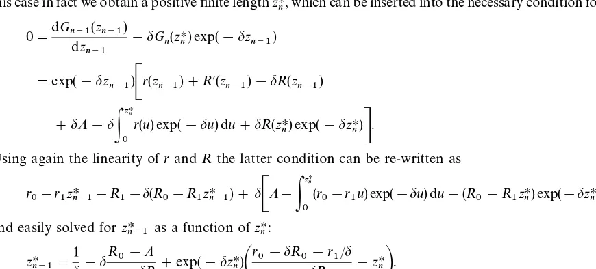
zHn"!R1!r0#dR0 this case in fact we obtain a positive"nite lengthzHn, which can be inserted into the necessary condition forzHn~1:
0"dGn~1(zn~1)
Using again the linearity ofrandRthe latter condition can be re-written as
r
Substituting forzHn, we getzHn~1and can proceed backward tozHs fors)n!2, according to the last formula of Section 6.
Example 4. We considern"3 cycles of a chain and assume the conditions given in Table 4. Using (7.1) and (7.2), the NPVG(z) turns out to be maximized at
z"[0, 4.926, 4.914, 5.667].
cycles. In particular, for the last cycle, we have a length of 5.667. The same e!ect can be noticed in the following example.
Example 5. We considern"20 cycles and adopt the speci"cations given in Table 5.
Using Eqs. (7.1) and (7.2), the NPVG(z) turns out to be maximized when the"rst"fteen cycles have length 8.124, with optimal length rapidly increasing (up to the last one, 13.581) after.
8. Conclusions and further research
This paper has extended the equivalent annuity de"nition}in the presence of a sequence of cycle investments}to the case of interest intensity variable over time.
It has examined"rst the correspondence/non correspondence of two procedures: maximizing (or minimiz-ing) the NPV directly or through the equivalent annuity.
Second, it has extended the ensuing optimization problem, with respect to the length of the cycles. As for the correspondence, we have argued that it holds}in an in"nite horizon framework}provided that we consider not the annuity over asingle cycleand the corresponding NPV, but the equivalent annuity over thewhole chainof cycles and its NPV. In the"nite horizon, the correspondence collapses also for thewhole chain(Section 3).
We have used a plant replacement model as an example (Section 4).
As for the optimal length problem, in the in"nite horizon case we have discussed both functional equation methods and Euler conditions (Section 5). In the"nite horizon one we have used recursive methods (Section 6). The latter have been applied to the plant replacement model (Section 7).
The plant replacement application is interesting not only per se, but also since it provides evidence of a substantial stationarity of the cycle lengths in su$ciently long chains. It also gives examples of optimal nonmonotonic policies.
The aforementioned stationarity of the optimal replacement policy even in"nite chains is currently under study. It holds under more general assumptions than the ones used in the examples of the present paper. It seems particularly promising for practical purposes, in that it indicates a simple, general structure for replacement policies, well grounded in theory. This general structure permits to understand better the implications of largely used approximations, such as the in"nite horizon one.
The main theoretical conclusion of the paper is that the equivalent annuity principle must be used with caution, whenever the model has optimization purposes, such as the choice of the optimal length of the NPV cycles. Our contribution consists exactly in pointing out the limits of its application and recalling methodolo-gies for the corresponding optimality problem.
The main practical contributions of the paper are three. First, lack of care in using equivalent annuities can be relevant in practice. In the plant replacement model example, for instance, we lose the 10}15% of net present value already during the"rst cycle, when using the equivalent annuity instead of the net present value. Furthermore, in one of our examples, the equivalent annuity produces a net loss, while net present value gives positive earnings. Second, our applications show that, under weak hypotheses, optimal replace-ment policies are approximately stationary even over a "nite horizon, which is somewhat surprising and interesting in itself. Last but not least, our setting is able to cope with the time evolution of interest rates, which these days is becoming more and more important also for non-"nancial users.
Acknowledgements
Appendix A.
In this appendix, with reference to the variabledcase, we prove that:
1. in the in"nite horizon case,maximizing(or minimizing)G
sis not the same as maximizing(or minimizing)Cs; 2. in the"nite horizon case,maximizing(or minimizing)GM is not the same as maximizing(or minimizing)CM.
Proof. 1. The"rst-order necessary condition forG
srequires that at interior (positive) stationary points, with
G
s di!erentiable, we have LG
s/Lzs"0. Fort
s~1 given, the"rst-order necessary condition on
C
In turn, this condition can be simpli"ed into
LG
s is not the same as maximizing(or minimizing)Cs.
2. The"rst-order necessary condition for a stationary point forGM andCM with respect toz
sare di!erent. The one forGM is
LGM /Lz
s"0 (A.1)
while, fort
s~1 given, the"rst-order necessary condition on
CM" GM
In turn, this condition can be simpli"ed into
Appendix B.
This appendix analyzes problem (P). Following Stokey and Lucas [10], we can de"neP(0), the set of admissible sequences of maturitiest
s, which are the nondecreasing ones, starting at 0:
P(0)"$ MMt
sN`s/0=: t0"0,ts`1*tss"0, 1,2N
and in generalP(t
0), the set of admissible (nondecreasing) sequences of maturitiests, starting fromt0*0:
P(t
0)"$ MMtsN`s/0=:ts`1*ts,s"0, 1,2N.
We denote with tI the elements ofP, i.e., those nondecreasing sequences which start att
0: MtsN`s/0="$ tI i! t
s`1*tsfor everys*0. On the setP(t0) we can de"ne the functionsun:P(t0)PR, partial sums of the series G, as follows:
u
n(tI)"$ n + s/1
H(t
s!ts~1)/(ts~1).
We can also de"ne their limit, as ndiverges:
u(tI)"$ lim n?`=
u
n(tI)
which mapsP(t
0) into the set of extended real numbersRM"$ RXM!R,#RN. Let us denote withvH(t0) the sup ofu(tI):
vH(t
0)"$ sup tI|P(
t0) u(tI)
which, by de"nition, exists, is unique and is the sup inP(the NPV once the optimal sequence of maturities has been chosen).
It can be proved (Theorems 4.2}4.5 of Stokey and Lucas [10]) thatvH(t
0) satis"es (5.1) and, conversely, that if there is a functionvwhich satis"es (5.1) and is such that
lim n?`=
v(t
n)"0
for every admissible sequencetI, thenvis the sup in problem (P):v"vH(t
0). In both cases the corresponding optimal timings, i.e. the ones that attain the supremum in (P), and which we denote withMtH
sN, satisfy
v(tH
s~1)"H(tHs!tHs~1)/(tHs~1)#v(tHs) (B.1) for everys. Conversely, every time sequencetI which satis"es (B.1) and has the property
lim s?`=
supv(tH
s))0
References
[1] D. Babusiaux, DeHcision d'Investissement et Calcul EDconomique dans l'Entreprise, Technip-Economica, Paris, 1990.
[2] P. Gallo, L. Peccati, The appraisal of industrial investments: A new method and a case study, International Journal of Production Economics 30}31 (1993) 465}476.
[3] R.W. GrubbstroKm, S.H. Ashcroft, Application of the calculus of variations to"nancing alternatives, Omega 19 (4) (1991) 305}316. [4] R.W. GrubbstroKm, A. Thorstenson, Principles for capital evaluation of inventory, Working paper No. 121, Department of
Production Economics, LinkoKping Institute of Technology.
[5] R.W. GrubbstroKm, A. Thorstenson, Evaluation of capital costs in a multi-level inventory system by means of the annuity stream principle, European Journal of Operational Research 24 (1) (1986) 136}145.
[6] E. Luciano, L. Peccati, Capital structure and inventory management: The temporary sale problem, 1996 ISIR Conference, Budapest, International Journal of Production Economics 59 (1998) 169}178.
[7] E. Luciano, L. Peccati, Some basic problems in inventory theory: The"nancial perspective. XV EURO and XXXIV INFORMS, Barcelona, 1998, European Journal of Operational Research 114 (1999) 294}303.
[8] L. Peccati, Multiperiod analysis of a levered portfolio, Riv. Mater. Sci. Econom. Soc. 12 (1) (1990) 157}166. [9] E. Schneider, Wahrscheinlichkeitsrechnung, Mohr, TuKbingen, 1951.
[10] N.L. Stokey, R.E. Lucas Jr., Recursive Methods in Economic Dynamics, Harvard University Press, Cambridge, MA, 1989. [11] A. Thorstenson, Capital Costs in inventory models}A Discounted Cash Flow Approach, PROFIL 8, Production-Economic
Research in LinkoKping, 1988.