www.elsevier.nlrlocaterjappgeo
Scattering attenuation: 2-D and 3-D finite difference simulations
vs. theory
Lena Frenje
), Christopher Juhlin
1Department of Earth Sciences, Uppsala UniÕersity, VillaÕagen 16, S-752 36 Uppsala, Sweden¨
Received 20 April 1999
Abstract
Ž .
Scattering of seismic waves is studied by producing synthetic vertical seismic profiling VSP seismograms with 2-D and 3-D finite difference modelling in random media. The random models used are Gaussian and band-limited self-similar, or fractal random media. The modelling is performed acoustically, but we believe that, considering the geometry of this study, the results obtained will hold for the elastic case as well.
Properties of the random media are discussed, in particular the difference between discrete and continuous media, and the importance of this difference. We show that when using the band-limited Von Karman correlation function when generating the random medium, the size of the model should be greater than 2pa, where a is the correlation distance, and the grid spacing should be less then a. If not, the medium will not have the proper characteristics.
Analytical expressions for scattering attenuation, derived from single scattering theory, can be used to estimate scattering
Q from borehole velocity logs, if it is known what minimum scattering angle,u , to use.u , the minimum angle energy,
min min
must be scattered to be regarded as not contributing to the propagating wave. We estimateumin by comparing Q values estimated from our synthetic VSP seismograms with the analytical expressions. The comparison also shows when the assumption of single scattering is valid. Previous studies in 2-D give aumin of;308. In this paper, we make a comparison for both the 2-D and 3-D cases, and show that the Q estimate is highly sensitive to how the analysis is done. We show that single scattering theory agrees well with finite difference simulations for self-similar media with low Hurst numbers, but with a somewhat lowerumin of 10–208. This holds for a range of correlation lengths, a, including the case of infinite, or absence of, a. For Gaussian and exponential media, simulations and theory agree as well withu of 10–208, but only for
min
ka-5, where k is the wave number of the source. For ka)5, simulations and theory diverge, and single scattering theory cannot explain the amplitude attenuation observed in the scattering simulations for these types of media, indicating that it may be difficult to estimate the fractal properties of a medium from seismic data alone.
With the difficulties of characterizing the scattering medium, and to estimate the scattering attenuation in the simple case of synthetic data with pure scattering, we conclude that it may be difficult to separate scattering and intrinsic attenuation from real data.q2000 Elsevier Science B.V. All rights reserved.
Keywords: Random media; Scattering attenuation; Finite differences; Single scattering theory
)Corresponding author. Fax:
q46-18-501110.
Ž . Ž .
E-mail addresses: [email protected] L. Frenje , [email protected] C. Juhlin .
1
Fax:q46-18-501110.
0926-9851r00r$ - see front matterq2000 Elsevier Science B.V. All rights reserved.
Ž .
1. Introduction
Over the past 15 years, scattering of seismic waves in random media in two dimensions has
Ž
been studied numerically Frankel and Clayton, 1984, 1986; Gibson and Levander, 1988; Ikelle
.
et al., 1993; Roth and Korn, 1993 . The random media generally consist of a deterministic back-ground velocity plus a random component de-fined by its wave number spectra. Gaussian, exponential and self-similar random media are often used in these scattering studies since these are easily defined by their respective wave num-ber spectra. Self-similar media, however, appear to best describe the spectral content of velocity
Ž
logs from boreholes Holliger, 1997; Dolan and
.
Bean, 1997; Leary, 1997 . Isotropic self-similar media are completely described by the standard deviation of the velocity fluctuations, correla-tion distance and Hurst number.
Analytical expressions for the amplitude de-cay of a forward propagating wave due to scat-tering may be estimated using single scatscat-tering
Ž .
theory Chernov, 1960 . An important parame-ter in the analytical expressions for scatparame-tering Q is u , the minimum angle that energy must be
min
scattered so as not to be considered as contribut-ing to the forward propagatcontribut-ing wave. At high wave numbers, 1rQ can vary by several orders
of magnitude depending upon the choice u .
min
In order to estimate scattering Q from borehole velocity logs it is, therefore, important to know what u to use in the analytical expressions.
min
Comparison of numerical simulations with the analytical functions is one method for determin-ing u . For 2-D media, Frankel and Clayton
min
Ž1986 and Roth and Korn 1993 estimated. Ž . u
min
to be about 308 for Gaussian and self-similar
Ž .
media. Sato 1982 derived a value of 298 from
a theoretical viewpoint.
In this paper, we perform a similar compari-son in 2-D as in the previous studies, but with significantly larger models and more synthetic data, which give better determined estimates. We also perform a 3-D comparison, which has not been done before, to investigate if a
differ-ence between 2-D and 3-D scattering simula-tions can be observed, or if 2-D is enough when studying scattering.
In the first part of this paper, we discuss the properties of random media and how they are generated. We will in detail investigate the dif-ferences between continuous and discrete media and point at the importance of this difference. In the second part, we generate synthetic
seismo-Ž .
grams for vertical seismic profiling VSP ac-quisition geometries in Gaussian and self-simi-lar 2-D and 3-D acoustic random media. The Hurst number and standard deviation of the velocity fluctuations of the random media are systematically varied. From the seismograms, we calculate the scattering attenuation observed in the finite difference seismograms and com-pare these results with analytical formulas
ŽChernov, 1960; Wu, 1982; Frankel and
Clay-.
ton, 1986 .
2. Random media
The random medium most often used to de-scribe heterogeneities in the crust is a spatially isotropic self-similar medium with a Gaussian probability density function, an autocovariance
Ž .
function N r and corresponding power
spec-Ž . Ž
trum P kr given by e.g., Frankel and Clayton,
.
where r is the spatial lag, s the standard
deviation of the velocity perturbations, a the correlation distance, n the Hurst number, G the
ns0.5, Eq. 1 corresponds to the well-known
exponential autocovariance function.
We generate our media in the wave number domain by creating a spectrum with a uniform, random phase between yp and p, and an
amplitude equal to the square root of the desired power spectrum, according to the
autocorrela-Ž .
tion theorem. Note that P 0 should be set to zero for a zero mean distribution. The final random medium is then obtained by inversely Fourier transforming the wave number spectrum to the spatial domain.
When generating the random medium, we believe it is common to scale the medium to the desired standard deviation as the last step. This can introduce an error since the standard devia-tion of a discrete medium differs from that of a continuous one, in some cases, quite
signifi-Ž .
cantly. Frankel and Clayton 1986 discuss this aspect for 2-D Gaussian and exponential media and the special case of 2-D self-similar media with a zero Hurst number. Here, we will gener-alise this concept for self-similar and Gaussian media in both two and three dimensions.
The standard deviation, s, can be calculated
in the wave number domain in 2-D and 3-D by
` `
spectively. In the discrete case, these integrals, or now rather the sums, will be truncated at the Nyquist frequency, causing the discrete standard deviation, s , to be less than the corresponding
d
continuous one. Further, since the size of the model is limited, the low wave numbers will not be present, further reducing s. That is, Eqs. 3
d
and 4 take the form 1
grid spacing. The sums over P are calculated by taking the average of neighbouring nodes. Fig. 1 shows hows varies with D in a model with a
d
fixed number of nodes. The decrease in s for
d
Ž .
larger D D)4 m in Fig. 1 is caused by the
truncation of the sum at the Nyquist wave
num-Ž
ber. The decrease in s for smaller D D-4
d .
m is caused by the limited size of the model, i.e., the loss of low wave numbers.
The reason for the reduction of s at the low
d
and high ends of the spectrum are of a com-pletely different nature. The ‘‘Nyquist decrease’’ is not an error, it is only the effect of going from the continuous to the discrete case.
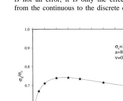
How-Fig. 1. The discrete standard deviation variation vs. grid
Ž . 3
spacing as predicted by Eq. 6 solid line in a model 128 nodes. Standard deviations observed in our random models
Žwith Ds0.5, 1.0, 2.0, 3.0, 4.0, 6.0 and 8.0 m are plotted.
ever, it is important to be aware of this differ-ence in order to obtain a discrete medium with the corresponding continuous properties. If the random medium is scaled at the end to the desired continuous standard deviation, this will result in a medium with the wrong character-istics. If the generation of the wave number spectrum and the inverse transform are done correctly, the standard deviations predicted by expressions 5 and 6 will fall out naturally, and should not be corrected for. The stars plotted in Fig. 1 show the standard deviations calculated from our random models without any scaling. There is a good agreement between the pre-dicted standard deviation and the observed stan-dard deviation in the model.
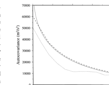
On the other hand, the decrease caused by the size of the model will result in a model with completely wrong characteristics. If the model is too small, the low wave numbers will be missing, along with the information about the correlation length. We calculated the power spectra and the autocorrelations of our models to check that we really had the characteristics that we wanted. In Fig. 2, the power spectra calculated from two models with the same pa-rameters and grid spacing but different sizes are
Ž 3 .
shown. The larger model 128 nodes is 12 times larger than the correlation length and the
3 Ž
Fig. 2. Power spectra for a model with 32 nodes black
. 3 Ž .
line and a model with 128 nodes grey, thick line .
Fig. 3. Autocorrelations of the same models as in Fig. 2
Ždotted line for the 323 model, dashed line for the 1283
.
model , in comparison with the theoretical correlation
Ž .
function solid line .
power spectrum shows both the flat part and the sloping fractal part, where the transition be-tween the two is determined by the correlation length, a, i.e., where kas1. On the other hand,
Ž 3 .
for the smaller model 32 nodes , which is only three times larger than the correlation length, the power spectrum only contains infor-mation about the fractal part and does not give any information about the correlation length. In Fig. 3, the theoretical correlation function given by Eq. 1 is plotted in comparison with the observed autocorrelations of the two models. These observed correlations are calculated by extracting several synthetic 1-D velocity logs from the models, calculating the autocorrela-tions for each log and then taking the average. The correlation curve from the smaller model deviates severely from the theoretical curve showing that this model does not have the de-sired characteristics. Our conclusions are that the size of the model must be large enough so that the minimum wave number, k s2prND,
min
is smaller than the corner wave number, kcs
1ra, i.e.,
ND)2pa
Ž .
7With the same argument as above, if the grid spacing is too large, no information about the sloping part of the power spectrum, and, thereby, the correlation length and the Hurst number will be present in the model. The grid spacing should be chosen at least so that the Nyquist wave number, k sprD is greater than k , i.e.,
Nyq c
D-pa. To get further constraints on how small D should be, we performed scattering
simula-tions in both self-similar and Gaussian media with varying D. The analysis of the simulations,
Ž .
which is presented later Comparison section , lead to the conclusion that one grid point per correlation length is enough for the medium to support the desired characteristics, i.e.,
DFa
Ž .
8However, the grid spacing is normally deter-mined by the velocity of the model and the frequency of the source to satisfy the dispersion requirements, so D will be <a.
3. Theoretical Q expressions
The theoretical expressions for the frequency dependence of Q are derived from single
scat-Ž .
tering theory, first presented by Chernov 1960 . Details of the derivation may be found in
Cher-Ž . Ž .
nov 1960 , Wu 1982 and Frankel and Clayton
Ž1986 . The relationship between inverse Q and.
the power spectrum of the random medium is,
2 p
is the 2-D power spectrum of the random medium and u is the minimum scattering
min
angle, i.e., the minimum angle that energy must be scattered to be regarded as not contributing to the propagating wave. Eq. 9 must be solved numerically.
For self-similar media, Eqs. 9 and 10 become
Qy2- D1
Ž .
kThe choice of u is very important, and it is
min
Ž .
not clear what value to use. Sato 1982 derived a value of 298 from a theoretical viewpoint. In
previous comparisons with numerical
simula-Ž
tions in 2-D Frankel and Clayton, 1986; Roth
.
and Korn, 1993 , a u of around 308 was
min
suggested. In this paper, we will make a similar comparison, both for the 2-D and 3-D case.
4. Synthetic data
We have generated synthetic VSP seismo-grams using a finite difference operator that is second order accurate in time and fourth order
Ž .
spectrum. Symmetric boundary conditions were implemented at all edges except at the top where a free surface was used. Since theoretical
scat-Ž .
tering Q is a function of ka Eqs. 11 and 12 , we kept the frequency content of the source constant and instead varied the correlation dis-tance. Thereby, we could use the same size for our models without changing the number of wavelengths the wave could propagate.
The sizes of our 2-D and 3-D models were 1666=2000 and 167=167=1333 grid points, respectively. The standard deviation of the ran-dom velocity fluctuations was 400 mrs super-imposed on a constant background velocity of 5000 mrs. We varied the correlation length from 5 to 160 m, and the Hurst number from 0.1 to 0.5 for the self-similar media. With a grid spacing of 3 m both expressions 7 and 8 are satisfied, and with a time step of 0.2 ms in 2-D and 0.15 ms in 3-D, the conditions for stability and numerical dispersion are satisfied.
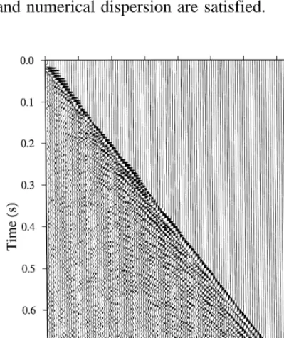
Fig. 4. One of the synthetic VSP seismograms recorded in a 3-D model with ss8%, ns0.1 and as40 m. The source is a plane Ricker wave with a dominant frequency of 80 Hz. The background velocity is constant at 5000 mrs.
Fig. 5. Peak amplitude vs. traveltime in synthetic VSP data
Ž . Ž .
from acoustic solid line and elastic dotted line model-ing.
About 100 evenly distributed VSP seismo-grams were recorded for each model, 48 m apart in the horizontal direction, in both 2-D and 3-D. No seismograms were recorded close to the edges to avoid possible edge effects. The downgoing wave was recorded every 33 m for each VSP. One example of a synthetic seismo-gram is plotted in Fig. 4. It shows a clear first arrival from the downgoing wave followed by scattered energy from the heterogeneities.
The modelling was performed acoustically, since it is computationally less expensive than elastic modelling, and we wanted to do a large number of simulations. In our case, with a plane wave and vertical incidence, the difference be-tween acoustic and elastic modelling should be minor. We carried out a 2-D elastic test run
ŽLevander, 1988 for comparison, and, as ex-.
pected, could not observe any major differences in the amplitude decay of the P-wave for the
Ž .
two types of modelling Fig. 5 . We believe that the results obtained in this paper hold for the elastic case as well.
5. Q value estimation
Fig. 6. The distribution of Q values calculated from the synthetic data described in Fig. 4.
giving an apparent Q for the model. Briefly, the method consists of comparing the peak ampli-tude of the downgoing wave at different depths.
The amplitude of a plane wave can be described
Ž .
by Aki and Richards, 1980
pf z
y
A z
Ž .
sA e0 QcŽ .
13 where Q is the number of wavelengths before the amplitude has been attenuated to eyp, or about 4% of its original value, f is the fre-quency of the wave, z is distance and c is wave velocity. Comparing the amplitudes at distance
z1 and z , assuming approximately constant2
velocity and taking the natural log, gives
pf
ln A z
Ž
Ž .
2.
yln A zŽ
Ž .
1.
s y DTŽ .
14Q
where DT is the traveltime from z to z . A
1 2
Ž .
plot of ln A vs. DT will yield a straight line,
where Q can be calculated from the slope. In
Ž .
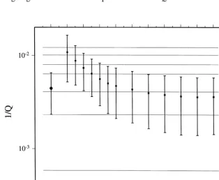
Fig. 7. 1rQ estimates squares from the same model as in Fig. 4 with error bars representing one standard deviation. Solid
Ž .
lines show values predicted by single scattering theory. The circle at zero window length shows the 1rQ estimate obtained
if no window is used, which corresponds to 1rQ being estimated in the time domain. The arrow indicates the 40-ms window
practice, the slope is determined by least squares. We did the Q estimation in the frequency do-main by applying a window around the first arrival and Fourier transforming the data. The apparent attenuation is then calculated with the peak amplitude method for the 80-Hz compo-nent, the dominant frequency of our source.
The calculation of Q is quite unstable, and, in many cases, several synthetic seismograms are generated and stacked prior to the analysis
Že.g., Korn, 1993 . However, stacking and esti-.
mating mean field attenuation can give the
Ž .
wrong result Sato, 1982; Wu, 1982 , and, in this study, we analysed each VSP seismogram individually, which resulted in a distribution of
Ž .
Q values for each model Fig. 6 . From this
distribution, we then calculated a mean value and a standard deviation, and compared it with what is predicted by single scattering theory.
The Q estimate is highly dependent on where in the model the seismogram is recorded. Gen-erally, the amplitude decay does not plot as a straight line but more chaotically. In some cases, the amplitude even increases with distance, re-sulting in a negative Q estimate. Further, quite different results can be obtained depending on how the analysis is done, as has been discussed
Ž
by several authors Sato, 1982; Wu, 1982;
.
Shapiro and Kneib, 1993 . The length of the window around the first arrival greatly affects
Ž .
the final Q estimate Shapiro and Kneib, 1993 . Fig. 7 shows the different results that can be obtained when varying the length of the win-dow. 1rQ is plotted vs. the window length
together with the predicted theoretical 1rQ
val-ues for some minimum scattering angles. In-creasing the window length results in that more scattered energy is included in the analysis and a lower 1rQ, i.e., a lower damping is observed.
In the following we have used a window length of 40 ms, 1.5 times the source wavelet length, to exclude the scattered coda and only account for the amplitude change in the first arrival. We also tried varying the tapering length of the window, but this did not have any influence on the final estimate.
6. Comparison
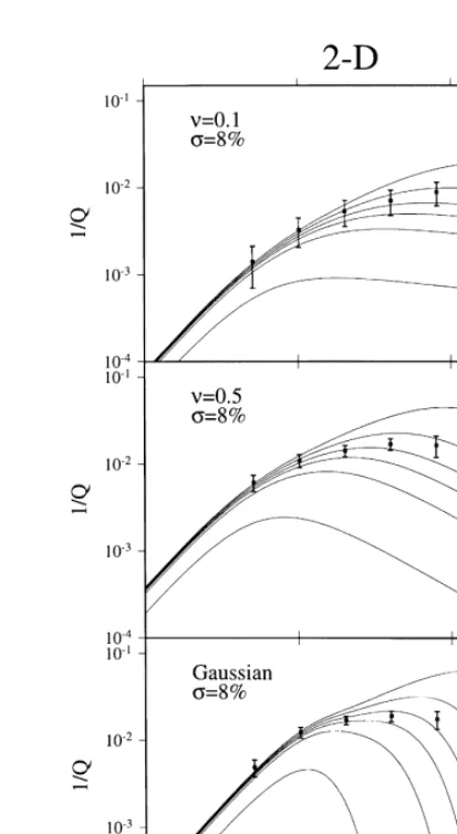
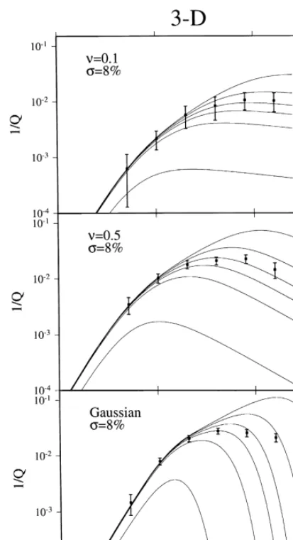
Figs. 8 and 9 show the comparison between theoretical Q values and the ones estimated from the numerical 2-D and 3-D simulations, respectively. In all cases, the Q estimates for
as5, 10, 20, 40, 80 and 160 m are plotted. Also plotted are the corresponding theoretical curves for various minimum scattering angles.
Fig. 8. Comparison between 1rQ estimates from 2-D
numerical simulations with error bars representing one
Ž .
standard deviation and theoretical 1rQ values thin lines . Ž .
The models are a self-similar medium top an exponential
Ž . Ž .
Fig. 9. Same type of plot as Fig. 8 but for the 3-D simulations.
In all cases, the simulations fall on the 10–208 u curves for ka-5. For ka)5, the
simula-min
tions deviate from the 10–208 curves for the
Gaussian and exponential medium, where a too high 1rQ is obtained compared to what is
predicted by theory. 1rQ remains almost
con-stant for ka)5. However, for the self-similar medium with ns0.1 the simulations still fall
on the 10–208 u curves. This is a somewhat
min
lower value for u than the 298 predicted
min
Ž .
theoretically by Sato 1982 and the 308
sug-gested by previous numerical simulations
ŽFrankel and Clayton, 1986, Roth and Korn,
.
1993 . We believe the difference between our results and the previous numerical simulations has two reasons. Firstly, as we stated earlier, the final Q estimate is highly sensitive to how the
Ž .
Q analysis is done. Frankel and Clayton 1986
used the peak amplitude method in the time domain after bandpass filtering the data. This is similar to not applying a window in our analysis
ŽFig. 7 . Sato 1982 did not include a window. Ž .
at all in his theoretical argument. Roth and Korn
Ž1993 applied a 90-ms window to their data.
and did the analysis for each frequency between 10 and 80 Hz. This means that the 10-Hz component will ‘‘see’’ a shorter window than the 80-Hz component and, according to Fig. 7, a lower 1rQ will be observed. To make a fair
comparison for different frequencies, different window lengths should be applied. We used a window corresponding to 1.5 times the source wavelet length, a 40-ms window. Using a larger window, or no window, would have given us a larger u . Secondly, the model size is of
im-min
Ž .
portance. Frankel and Clayton 1986 report that a random model of 17 wavelengths is enough to obtain accurate estimates of Q. Roth and Korn
Ž1993 used only. ;10 wavelengths. We be-lieve this is too small. With such a small model, varying the random seed of the random number generator can change the results significantly. In our simulations, we used a 6-km-deep model in 2-D and a 4-km-deep one in 3-D, and did the analysis over a depth range corresponding to 90 and 55 wavelengths, respectively. With these model sizes, we obtained stable Q estimates.
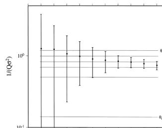
We also tried varying s, the velocity
stan-dard deviation of the random models, to see if this influenced the choice of the minimum scat-tering angle. We did the simulation in 2-D with
as40 m, ns0.1, and varied s between 2%
and 20%. Since the models with high s could
Fig. 10. 1rQ estimates from 2-D numerical simulations with as40 m,ns0.1 and varying standard deviation, s. The source is a plane Ricker wave with a dominant frequency of 50 Hz.
s2
to allow a direct comparison. It is clear that the choice of u depends strongly on s.
min
However, the smaller s, the larger the error
bars since a medium close to homogeneous will only slightly attenuate the wave and, therefore, the Q estimate is quite unstable. This s
depen-dence might also explain the difference between our results and those that Frankel and Clayton
Ž1986 obtained. They used a higher. s Ž10% in.
their models than we did.
When comparing Figs. 8 and 9, no major differences between the 2-D and 3-D simula-tions can be observed. However, we noticed that the 2-D simulations had larger standard devia-tions than the 3-D simuladevia-tions when the models had the same depths. That is, 3-D simulations appear to be more stable than 2-D. Using a 6-km-deep 2-D model and a 4-km-deep 3-D model resulted in roughly the same standard deviations.
As mentioned in the Random media section, we also did some simulations to obtain
con-straints on the choice of the grid spacing, D. We
did the simulations in 2-D for both self-similar and Gaussian media, with as5 m, ss8%,
Fig. 11. 1rQ estimates in media with varying grid
and varied D between 1 and 10 m. The source
was a 80-Hz Ricker wavelet. The result is plot-ted in Fig. 11. Roughly the same 1rQ estimate
is obtained for D-1.5a, but for D)1.5a, the
1rQ estimates starts deviating. We conclude
that with DFa, the random model will support
the desired characteristics, such as correlation length and Hurst number. It is somewhat sur-prising that the grid spacing can be on the same order as a, and a stable estimate of 1rQ can be
obtained. This may be due to that the dominant wavelength used in these simulations was ap-proximately 60 m, and, therefore, was insensi-tive to variations on the order of 5 m.
7. Discussion
The deviation from the 10–208 u curves
min
for high ka in Figs. 8 and 9 for Gaussian and exponential media could be caused by multi-pathing or multiple scattering, explanations that have been mentioned earlier by both Frankel
Ž . Ž .
and Clayton 1986 and Roth and Korn 1993 . The authors suggested that larger models might improve the results. We tried using larger mod-els, but our results were the same in the high ka range. The only difference was that the standard deviation decreased, the mean value remained the same. We believe that the deviation is caused by the fact that single scattering is not valid in the high ka range for Gaussian and exponential
Ž .
media. Levander et al. 1994 show a scattering
Ž .
regime diagram Fig. 5 in their paper where
Ž . Ž .
log ka ylog Lra space, L is path length, is
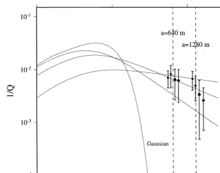
divided into different regions with different types of scattering. All our simulations fall into the weak scattering region, i.e., single scattering should dominate. The simulations with low ka fall into the subpart of the weak scattering region that can be explained by classical scatter-ing, whereas the simulations with high ka ap-proach the geometrical optics part where scatter-ing is not relevant. We did some simulations in 2-D for the different models with very large
correlation lengths, as640 m on a 10=6-km model, and as1280 m on a 12=12-km model. These simulations are well within the geometri-cal optics part. The results are shown in Fig. 12 together with theoretical curves for u s108.
min
For the self-similar medium, with ns0.1, the
simulations still agree with single scattering the-ory. However, for the self-similar media with higher Hurst numbers, as well as for the Gauss-ian medium, simulations and theory diverge and single scattering theory cannot explain the atten-uation observed in these cases.
In Gaussian and exponential media, the corre-lation length corresponds to the characteristic scale of the heterogeneities, or ‘‘blobbs’’, in the model. A large value of a means large blobbs, and the energy will be mainly reflected at the blobbs, not scattered. This means that the wave-field, and, thereby, Q, will be sensitive only to the velocity contrast in the model, and not what type of medium it is. However, for self-similar media with low Hurst numbers, scattering is relevant in the high ka range as well. This type of medium does not have a characteristic scale, and small-scale heterogeneities, causing scatter-ing, will be present in the model, independently of a. A low Hurst number will also mean a high content of small-scale heterogeneities. We did some simulations in models with a low Hurst number and infinite, or absence of, correlation length, i.e., media that are fractal on all scales, and the estimated 1rQ still agreed well with
single scattering theory for a u of 10–208.
min
The finite difference modelling in this study shows that the observed Q is dependent upon the choice of all three parameters, s, n and a.
Analyses of the amplitude decay of first arrivals in VSP data could provide information on these parameters. However, there are a couple of problems that must be dealt with prior to any ‘‘inversion’’ attempt. Firstly, the physical sig-nificance of a in real rocks must be further
Ž .
Ž . Ž .
Fig. 12. 1rQ estimates from 2-D numerical simulations in self-similar models with ns0.1 squares , ns0.3 stars ,
Ž . Ž .
ns0.5 circles and Gaussian models diamonds , with correlation lengths of 640 and 1280 m. For visualization, the
estimates are spread out slightly sideways around the dotted lines, which indicate the true position of the estimates. Theoretical curves foru s108are also plotted.
min
Ž .
infinite Dolan and Bean, 1997; Leary, 1997 , i.e., the variations in velocity are scale indepen-dent. The practical limit for a may be the
Ž .
thickness of the crust Dolan and Bean, 1997 . However, our study shows that in the case of a self-similar medium with a low Hurst number, single scattering theory can successfully predict the scattering attenuation observed, indepen-dently of a, so, from the simulation point of view, an infinite a need not be a problem. Secondly, the observed amplitude decay is highly dependent on the location of the borehole in the random media. Some locations will give a
Ž .
strong amplitude decay low Q , while others
Ž
may even give an amplitude increase negative
.
Q . Since generally only one borehole, or at
best a few boreholes, are available in a given area, caution should be used when interpreting scattering Q from VSP data.
Finally, since single scattering theory cannot predict the 1rQ estimates obtained for high ka
in our simulations, and sometimes quite similar values can be obtained for the different models, it is not possible to discriminate between the different types of random media in this range. To be able to discriminate a self-similar medium from an exponential or a Gaussian one, ka must be less than ;5. Unfortunately, the difference between predicted 1rQ values for the different
types of media is small in the low ka range, indicating the difficulty in extracting informa-tion about the type of media from only seismic data.
attenuation from real data will most likely be very difficult.
8. Conclusions
When generating random media, the differ-ence between continuous and discrete media must be taken into account. The standard devia-tion of a discrete medium can be decreased to 50% of that of the corresponding continuous medium. Not considering this effect will intro-duce major errors in the characteristics of the medium.
The calculation of scattering Q is highly sensitive to how the analysis is done. The length of the window around the first arrival highly affects the final Q estimate, and almost any choice of minimum scattering angle between 108and 308is reasonable. With our analysis, we
find that theoretical scattering Q, derived from single scattering theory, agrees well with results from 2-D and 3-D finite difference simulations for ka-5 in Gaussian and exponential media, and for all ka in self-similar media with low Hurst numbers, even in the case of infinite a. The best match is obtained for a minimum scattering angle of ;10–208 in all cases when
a window length of 1.5 times the source wavelet length is used. However, for ka)5, theory and simulations diverge in Gaussian and exponential media, implying that single scattering theory cannot explain the amplitude attenuation ob-served, and it is not possible to discriminate between the different types of media for high ka in scattering experiments. Further, the choice of
u depends on s, the standard deviation of
min
the velocity variations, with an increase of u
min
when s increases.
With the difficulties of estimating the scatter-ing attenuation in the simple, synthetic cases with pure scattering that we investigated in this study, we believe it will be difficult to separate scattering and intrinsic attenuation from real data.
No major differences between the 2-D and 3-D simulations could be observed, except that the 3-D simulations appeared to be more stable with smaller standard deviations for the Q esti-mates.
Acknowledgements
We thank Klaus Holliger and an anonymous reviewer for comments that improved this pa-per. C. Juhlin is funded by the Swedish Natural
Ž .
Science Research Council NFR . Computer time on a parallel IBM SP was provided by the Center for Parallel Computers at the Royal Insti-tute of Technology in Stockholm.
References
Aki, K., Richards, P.G., 1980. Quantitative Seismology. Freeman, 167 pp.
Alford, R.M., Kelly, K.R., Boore, D.M., 1974. Accuracy of finite difference modelling of the acoustic wave equation. Geophysics 39, 834–841.
Chernov, L.A., 1960. Wave Propagation in a Random Medium. McGraw-Hill, New York, NY.
Dolan, S., Bean, C., 1997. Some remarks on the estimation of fractal scaling parameters from borehole wire-line logs. Geophys. Res. Lett. 24, 1271–1274.
Frankel, A., Clayton, R.W., 1984. A finite difference simulation of wave propagation in two-dimensional random media. Bull. Seismol. Soc. Am. 74, 2167–2186. Frankel, A., Clayton, R.W., 1986. Finite difference simula-tions of seismic scattering: implicasimula-tions for the propa-gation of short-period seismic waves in the crust and models of crustal heterogeneity. J. Geophys. Res. 91, 6465–6489.
Gibson, B.S., Levander, A.R., 1988. Modeling and pro-cessing of scattered waves in seismic reflection sur-veys. Geophysics 53, 466–478.
Holliger, K., 1996. Upper-crustal seismic velocity hetero-geneity as derived from a variety of P-wave sonic logs. Geophys. J. Int. 125, 813–829.
Holliger, K., 1997. Seismic scattering in the upper crys-talline crust based on evidence from sonic logs. Geo-phys. J. Int. 128, 65–72.
Korn, M., 1993. Seismic waves in random media. J. Appl. Geophys. 29, 247–269.
Leary, P.C., 1997. Relating microscale rock–fluid interac-tion to macroscale fluid flow structure. In: Leeds96 Fault Seal Conference — 29Oct96. In press.
Levander, A.R., 1988. Fourth-order finite-difference P-SV seismograms. Geophysics 53, 1425–1436.
Levander, A.R., Hobbs, R.W., Smith, S.K., England, R.W., Snyder, D.B., Holliger, K., 1994. The crust as a hetero-geneous ‘‘optical’’ medium, or ‘‘crocodiles in the mist’’. Tectonophysics 232, 281–297.
Roth, M., Korn, M., 1993. Single scattering theory versus numerical modelling in 2-D random media. Geophys. J. Int. 112, 124–140.
Sato, H., 1982. Amplitude attenuation of impulsive waves in random media based on travel time corrected mean wave formalism. J. Acoust. Soc. Am. 71, 559–564. Shapiro, S.A., Kneib, G., 1993. Seismic attenuation by
scattering: theory and numerical result. Geophys. J. Int. 114, 373–391.