Justi
"
cation of manufacturing technologies using fuzzy
bene
"
t/cost ratio analysis
Cengiz Kahraman
!,
*, Ethem Tolga
"
, Ziya Ulukan
"
!Department of Industrial Engineering, Istanbul Technical University 80680 Mac7ka-Istanbul, Turkey"Faculty of Engineering and Technology, Galatasaray University, 80840 Ortakoy-Istanbul, Turkey
Received 23 June 1998; accepted 15 July 1999
Abstract
The application of discounted cash#ow techniques for justifying manufacturing technologies is studied in many papers. State-price net present value and stochastic net present value are two examples of these applications. These applications are based on the data under certainty or risk. When we have vague data such as interest rate and cash#ow to apply discounted cash#ow techniques, the fuzzy set theory can be used to handle this vagueness. The fuzzy set theory has the capability of representing vague data and allows mathematical operators and programming to apply to the fuzzy domain. The theory is primarily concerned with quantifying the vagueness in human thoughts and perceptions. In this paper, assuming that we have vague data, the fuzzy bene"t}cost (B/C) ratio method is used to justify manufacturing technologies. After calculating theB/Cratio based on fuzzy equivalent uniform annual value, we compare two assembly manufacturing systems having di!erent life cycles. ( 2000 Elsevier Science B.V. All rights reserved.
Keywords: Economic justi"cation; Fuzzy set theory;B/Cratio
1. Introduction
Many authors give the economic justi"cation
approaches of manufacturing systems: Meredith and Suresh [1], Lavelle and Liggett [2], Soni et al. [3], Kolli et al. [4], Boaden and Dale [5], Khouja
and O!odile [6], Proctor and Canada [7], etc.
Kolli et al. [4] classify the approaches into two main groups: single criterion and multi-criteria approaches. These two main groups are then divided into two subgroups: deterministic and non-deterministic approaches. Simple criterion and
*Corresponding author.
E-mail addresses:[email protected] (C. Kahra-man), [email protected] (E. Tolga)
deterministic approaches contain discounted cash
#ow techniques (NPV, JRR, PP, etc.). Single
cri-terion and nondeterministic approaches contain sensitivity analysis, decision tree, Monte Carlo simulation, etc. Multi-criteria deterministic ap-proaches contain scoring, AHP, goal program-ming, DSS, dynamic programprogram-ming, and ranking
methods (ELECTRE, PROMETHEE,2).
Multi-criteria nondeterministic approaches contain fuzzy linguistics, expert system, utility models, and game theoretic models. Wilhelm and Parsaei [8] use a fuzzy linguistic approach to justify a
computer-integrated manufacturing system. Kahraman
et al. [9] use a fuzzy approach based on the fuzzy present value analysis for the manufacturing
#exibility.
To deal with vagueness of human thought,
Zadeh [10], "rst introduced the fuzzy set theory,
which was oriented to the rationality of uncertainty due to imprecision or vagueness. A major contribu-tion of fuzzy set theory is its capability of repres-enting vague data. The theory also allows mathematical operators and programming to ap-ply to the fuzzy domain. A fuzzy set is a class of objects with a continuum of grades of membership. Such a set is characterized by a membership (char-acteristic) function, which assigns to each object a grade of membership ranging between zero and one.
Quite often in"nance future cash amounts and
interest rates are estimated. One usually employs educated guesses, based on expected values or other statistical techniques, to obtain future cash
#ows and interest rates. A statement like`
approx-imately between 10% and 15%amust be translated
into an exact amount such as`12.5%a.
Appropri-ate fuzzy numbers can be used to capture the
vagueness of `approximately between 10% and
15%a[11].
A tilde&&'will be placed above a symbol if the
symbol represents a fuzzy set. Therefore,PI,r8,n8 are
all fuzzy sets. The membership functions for these
fuzzy sets will be denoted by k(xDPI), k(xDr8), and
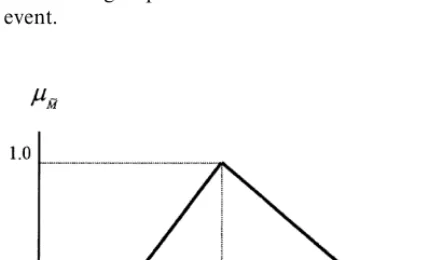
k(xDn8) respectively. A triangular fuzzy number
(TFN), MI is shown in Fig. 1. A TFN is denoted
simply as (m
1/m2,m2/m3) or (m1, m2, m3). The
parametersm
1,m2andm3respectively denote the
smallest possible value, the most promising value, and the largest possible value that describe a fuzzy event.
Fig. 1. A triangular fuzzy number,MI .
Each TFN has linear representations on its left and right side such that its membership function
can be de"ned as
A fuzzy number can always be given by its corre-sponding left and right representation of each degree of membership:
MI "(M-(y),M3(y))
"(m
1#(m2!m1)y,m3#(m2!m3)y)
∀y3[0, 1], (2)
where l(y) and r(y) denotes the left side representa-tion and the right side representarepresenta-tion of a fuzzy number, respectively. Zimmermann [12] gives the algebraic operations with triangular fuzzy num-bers. Many ranking methods for fuzzy numbers have been developed in the literature. They do not necessarily give the same rank. Two ranking methods are given in the appendix.
Buckley [11], Ward [13], Chiu and Park [14], Wang and Liang [15], Kahraman and Tolga [16] are among the authors who deal with the fuzzy
present worth analysis, the fuzzy bene"t/cost ratio
analysis, the fuzzy future value analysis, the fuzzy payback period analysis, and the fuzzy capitalized value analysis.
2. Fuzzy bene5t/cost ratio analysis
The bene"t}cost ratio can be de"ned as the ratio
of the equivalent value of bene"ts to the equivalent
value of costs. The equivalent values can be present values, annual values, or future values. The
bene-"t}cost ratio (BCR) is formulated as
BCR"B/C, (3)
whereBrepresents the equivalent value of the
be-ne"ts associated with the project andCrepresents
the project's net cost [17]. AB/Cratio greater than
In B/C analyses, costs are not preceded by a minus sign. The objective to be maximized behind
the B/C ratio is to select the alternative with the
largest net present value or with the largest net
equivalent uniform annual value, because B/C
ra-tios are obtained from the equations necessary to
conduct an analysis on the incremental bene"ts and
costs. Suppose that there are two mutually exclus-ive alternatexclus-ives. In this case, for the incremental
BCR analysis ignoring disbene"ts the following
ratios must be used:
2v1 is the incremental bene"t of
Alterna-tive 2 relaAlterna-tive to AlternaAlterna-tive 1, *C
2v1 is the
in-cremental cost of Alternative 2 relative to
Alternative 1,*PVB
2v1is the incremental present
value of bene"ts of Alternative 2 relative to
Alter-native 1,*PVC
2v1is the incremental present value
of costs of Alternative 2 relative to Alternative1, *EUAB
2v1 is the incremental equivalent uniform
annual bene"ts of Alternative 2 relative to
Alterna-tive 1 and*EUAC
2v1is the incremental equivalent
uniform annual costs of Alternative 2 relative to Alternative 2.
Thus, the concept ofB/Cratio includes the
ad-vantages of both NPV and NEUAV analyses. Because it does not require to use a common
mul-tiple of the alternative lives (then B/Cratio based
on equivalent uniform annual cash #ow is used)
and it is a more understandable technique relative to rate of return analysis for many
"nancial managers, B/C analysis can be preferred to the other techniques such as present value analysis, future value analysis, rate of return analysis.
In the case of fuzziness, the steps of the fuzzyB/C
analysis are given in the following:
Step 1: Calculate the overall fuzzy measure of bene"t-to-cost ratio and eliminate the alternatives
that have
wherer8 is the fuzzy interest rate and r(y) and l(y) are
the right and left side representations of the fuzzy
interest rates and 13 is (1, 1, 1), andnis the crisp life
cycle.
Step 2: Assign the alternative that has the lowest initial investment cost as the defender and the next-lowest acceptable alternative as the challenger.
Step 3: Determine the incremental bene"ts and the incremental costs between the challenger and the defender.
Step 4: Calculate the *BI/*CI ratio, assuming that the largest possible value for the cash in year
t of the alternative with the lowest initial
invest-ment cost is less than the least possible value for the
cash in yeartof the alternative with the next-lowest
initial investment cost.
The fuzzy incremental BCR is
*BI
ratio of a single investment alternative is
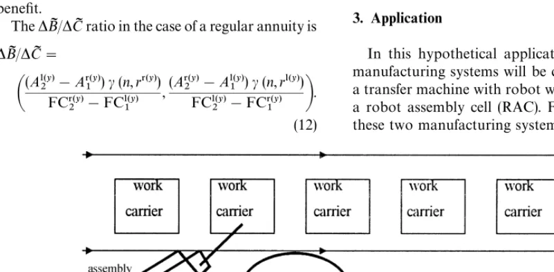
Fig. 2. RW*transfer machine with robot workhead. Step 5: Repeat steps 3 and 4 until only one
alternative is left, thus the optimal alternative is obtained.
The cash-#ow set MA
t"A:t"1, 2,2,nN,
con-sisting ofncash#ows, each of the same amountA,
at times 1, 2,2,n, with no cash#ow at time zero, is
called the equal-payment series. An older name for it is the uniform series, and it has been called an
annuity, since one of the meanings of `annuityais
a set of "xed payments for a speci"ed number of
years. To "nd the fuzzy present value of a regular
annuity MAIt"AI:t"nN, we will use Eq. (10). The
membership functionk(xDPIn) forPInis determined by
f
ni(yDPIn)"fi(yDAI )c(n,f3~i(yDr8)) (10)
for i"1, 2 and c(n,r)"(1!(1#r)~n)/r. Both
AI andr8 are positive fuzzy numbers.f
1(.) and f2(.) shows the left and right representations of the fuzzy numbers, respectively.
In the case of a regular annuity, the fuzzy BI/CI
ratio may be calculated as in the following:
The fuzzyBI/CI ratio of a single investment
alter-native is
Up to this point, we assumed that the alterna-tives had equal lives. When the alternaalterna-tives have
life cycles di!erent from the analysis period, a
com-mon multiple of the alternative lives (CMALs) is calculated for the analysis period. Many times, a CMALs for the analysis period hardly seems
realistic (CMALs (7, 13)"91 years). Instead of an
analysis based on present value method, it is
appro-priate to compare the annual cash#ows computed
for alternatives based on their own service lives. In
the case of unequal lives, the following fuzzy BI/CI
and*BI/*CI ratios will be used:
where PVB is the present value of bene"ts, PVC the
present value of costs and
b(n,r)"((1#n)ni/((1#r)n!1)).
3. Application
Table 1
The fuzzy data for RAC Year,t Revenue ($)
REV3t(]103)
Labour cost ($) LAB3t(]103)
Investment ($)
II
t(]103)
Depreciation ($) DEP3t(]103)
After-tax cash#ow ($) ATCF3t(]103)
1 (180, 200, 220) (60, 70, 80) (270, 280, 290) (50, 60, 70) (!210,!178,!146) 2 (200, 210, 220) (65, 75, 85) (7, 8, 9) (45, 50, 55) (78, 93, 108)
3 (220, 230, 240) (70, 80, 90) (7, 8, 9) (35, 40, 45) (83, 98, 113) 4 (320, 330, 340) (105, 115, 125) (25, 30, 40) (35, 40, 45) (91, 115, 134) 5 (350, 360, 370) (115, 120, 125) (10, 15, 20) (30, 35, 40) (127, 143, 161) 6 (390, 400, 410) (130, 135, 140) (300, 310, 320) (80, 85, 90) (!138,!117,!96) 7 (425, 430, 435) (140, 150, 160) (20, 25, 30) (70, 75, 80) (157, 173, 189)
Table 2
The calculatedA¹CFItfor RW
Year,t 1 2 3 4 5
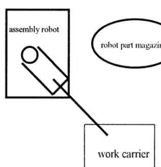
ATCF3t(]103$) (!190,!128,!94) (109, 130, 151) (116, 137, 158) (127, 161, 187) (178, 200, 225) Fig. 3. RAC*robot assembly cell.
The robot assembly cell uses one robot. This sophisticated robot has six degrees of freedom. Tables 1 and 2 give the data for RAC and RW, respectively. The tax rate (TR) is 40% and is not fuzzy. The crisp life cycles are 7 years for RAC and 5 years for RW. The fuzzy discount rate is (15%, 20%, 25%) per year.
To fuzzify the data for RAC and RW, it is as-sumed that the model parameters are triangular fuzzy numbers. The parameters like the average
time for the robot to assemble a part, the part quality, the average downtime at a station due to a defective part, the number of production hours
per shift, the plant e$ciency, the cost of a robot, the
cost of a part feeder, the cost of a robot gripper, the annual cost of a supervisor have been accepted as triangular fuzzy numbers. For example, the average
time of the RAC to complete an assemblyi, is used
while calculating the number of shifts and the an-nual labour cost. It is formulated by
AT3
i"NP3i?[AP3 =PQ3 ?AD3 ], (15)
where NP3
i is the fuzzy number of parts in each
assemblyi, AP3 the fuzzy average time (in seconds)
for the robot to assemble one part, PQ3 the fuzzy
part quality (the fraction of defective parts to good
parts), and AD3 the fuzzy average downtime at a
station due to a defective part.
The other details are not given in the paper but the calculated results are.
In year 6, a new robot assembly cell is required.
So, ATCF3
6(0. While calculating after-tax cash
#ow, the following formula has been used:
ATCF3
t"(REV3t!LAB3t)(1!TR)
=DEP3
Now, using Eq. (13), we will calculateBI/CI ratios
for each alternative. First, let us calculate PVB3
RAC,
The approximate forms of PVB3
RW, PVB3RAC,
PVC3
RW, and PVC3RACare found as in the following,
takingy"0, 1 and 0, respectively:
PVB3
RAC"$(204.230, 282.505, 383.675),
PVB3
RW"$(239.498, 327.578, 436.848),
DPVC3
RACD"$(153.817, 194.549, 233.191),
DPVC3
RWD"$(81.739, 106.667, 165.217),
PVB3
RAC"(78.275y#204.230, 383.675!101.17y),
PVB3
RW"(88.08y#239.498, 436.848!109.27y),
DPVC3
RACD"(40.732y#153.817, 233.191!38.642y)
DPVC3
RWD"(24.928y#81.739, 165.217!58.55y),
<"
C
(1.15#0.05y)5(0.15#0.05y)RW"(1.163, 3.071, 6.662),
*BI"(!113.352,!31.162, 49.926),
*CI"(!24.464, 18.305, 49.384),
*BI/*CI"(!2.295,!1.702, 2.041),
*BI/*CI"(a,b,c).
Kaufmann and Gupta's ranking method:
(a#2b#c)/4"!0.915,
13"(1, 1, 1),
*BI/*CI (13, then the preferred alternative is RW.
Chiu and Park's weighting method (w"0.3):
((a#b#c)/3)#wb"!1.16, 13"(1, 1, 1),
((a#b#c)/3)#wb"1.3,
*BI/*CI (13, then the preferred alternative is RW.
4. Conclusions
This paper develops a fuzzyB/Cratio analysis to
justify a manufacturing technology. The analysis presents an alternative to having to use exact
amounts for the parameters used in the justi"cation
process. Fuzzy B/Cratio analysis is equivalent to
fuzzy present value analysis. However, fuzzy B/C
ratio based on equivalent uniform annual bene"ts
and costs has the advantage of comparing
alterna-tives having life cycles di!erent from the analysis
period, without calculating a common multiple of
the alternative lives. The details of fuzzyB/Cratio
are presented in this paper.
The developed fuzzy B/C ratio analysis only
takes into account of a quantitative criterion that is
the pro"tability, while justifying a manufacturing
technology. To justify a manufacturing technology, generally, a number of quantitative and qualitative criteria have to be considered. In this case, deter-ministic or nondeterdeter-ministic multiple criteria methods such as scoring or fuzzy linguistics should be taken into account.
Appendix
There are a number of methods that are devised
to rank mutually exclusive projects such as Chang's
method [18], Jain's method [19], Dubois and
Prade's method [20], Yager's method [21], Baas
and Kwakernaak's method [22]. However, certain
shortcomings of some of the methods have been
reported in [23}25]. Because the ranking methods
might give di!erent ranking results, they must be
used together to obtain the true rank. Chiu and Park [14] compare some ranking methods by using a numerical example and determine which methods
give the same or very close results to one another.
In Chiu and Park's [14] paper, several dominance
methods are selected and discussed. Most methods are tedious in graphic manipulation requiring
com-plex mathematical calculation. Chiu and Park's
weighting method and Kaufmann and Gupta's
[26] three criteria method are the methods giving the same rank for the considered alternatives and these methods are easy to calculate and require no graphical representation. Therefore, these two methods will be explained in the following and will be used in the application section.
Chiu and Park's [14] weighted method for
ranking TFNs with parameters (a,b,c) is
for-mulated as
((a#b#c)/3)#wb,
wherewis a value determined by the nature and the
magnitude of the most promising value.
Kaufmann and Gupta [26] suggest three criteria
for ranking TFNs with parameters (a,b,c). The
dominance sequence is determined according to priority of:
1. comparing the ordinary number (a#2b#c)/4,
2. comparing the mode (the corresponding most
promising value),b, of each TFN,
3. comparing the range,c}a, of each TFN.
The preference of projects is determined by the amount of their ordinary numbers. The project with the larger ordinary number is preferred. If the ordinary numbers are equal, the project with the larger corresponding most promising value is pre-ferred. If projects have the same ordinary number and most promising value, the project with the larger range is preferred.
References
[1] J.R. Meredith, N.C. Suresh, Justi"cation techniques for advanced manufacturing technologies, International Jour-nal of Production Research 24 (5) (1986) 1043}1058. [2] J.P. Lavelle, H.R. Liggett, Economic methods for
[3] R.G. Soni, H. Parsaei, D.H. Liles, Economic and"nancial justi"cation methods for advanced automated manufac-turing: an overview, in: H.R. Parsaei, A. Mital (Eds.), Economics of Advanced Manufacturing Systems, Chap-man & Hall, London, 1992.
[4] S. Kolli, M.R. Wilhelm, D.H. Liles, A classi"cation scheme for traditional and non-traditional approaches to the eco-nomic justi"cation of advanced automated manufacturing systems, in: H.R. Parsaei, W.G. Sullivan, T.R. Hanley (Eds.), Economic and Financial Justi"cation of Advanced Manufacturing Technologies, Elsevier, Amsterdam, 1992, pp. 165}187.
[5] R.J. Boaden, B. Dale, Justi"cation of computer-integrated manufacturing: some insights into the practice, IEEE Transactions on Engineering Management 37 (4) (1990) 291}296.
[6] M. Khouja, O.F. O!odile, The industrial robot selection problem: Literature review and directions for future research, IIE Transactions 26 (4) (1994) 50}61.
[7] M.D. Proctor, J.R. Canada, Past and present methods of manufacturing investment evaluation: A review of the empirical and theoretical literature, The Engineering Eco-nomist 38 (1) (1992) 45}58.
[8] M.R. Wilhelm, H.R. Parsaei, A fuzzy linguistic approach to implementing a strategy for computer integrated manufacturing, Fuzzy Sets and Systems 42 (1991) 191}204.
[9] C. Kahraman, E. Tolga, Z. Ulukan, Fuzzy#exibility analy-sis in automated manufacturing systems, Proceedings of INRIA/IEEE Conference on Emerging Technologies and Factory Automation, Vol. 3, October 10}13, Paris, 1995, pp. 299}307.
[10] L.A. Zadeh, Fuzzy sets, Information and Control 8 (1965) 338}353.
[11] J.U. Buckley, The fuzzy mathematics of"nance, Fuzzy Sets and Systems 21 (1987) 257}273.
[12] H.-J. Zimmermann, Fuzzy Set Theory and its Applica-tions, Kluwer Publishing, Dordrecht, 1994.
[13] T.L. Ward, Discounted fuzzy cash#ow analysis, Proceed-ings of 1985 Fall Industrial Engineering Conference, Insti-tute of Industrial Engineers (1985) 476}481.
[14] C. Chui, C.S. Park, Fuzzy cash#ow analysis using present worth criterion, The Engineering Economist 39 (2) (1994) 113}138.
[15] M.-J. Wang, G.-S. Liang, Bene"t/cost analysis using fuzzy concept, The Engineering Economist 40 (4) (1995) 359}376. [16] C. Kahraman, E. Tolga, The e!ects of fuzzy in#ation rate on after-tax rate calculations, third Balkan Conference on Operational Research, Thessaloniki, Greece, 16}19 Octo-ber 1995.
[17] L.T. Blank, J.A. Tarquin, Engineering Economy, 3rd Edition, McGraw-Hill, Inc., New York, 1989.
[18] W. Chang, Ranking of fuzzy utilities with triangular mem-bership functions, Proceedings of the International Con-ference of Policy Anal. and Inf. Systems, 1981, pp. 263}272. [19] R. Jain, Decision-making in the presence of fuzzy vari-ables, IEEE Transactions on Systems, Man, and Cyber-netics 6 (1976) 693}703.
[20] D. Dubois, H. Prade, Ranking fuzzy numbers in the setting of possibility theory, Information Sciences 30 (1983) 183}224.
[21] R.R. Yager, On choosing between fuzzy subsets, Kyber-netes 9 (1980) 151}154.
[22] S.M. Baas, H. Kwakernaak, Rating and ranking multiple-aspect alternatives using fuzzy sets, Automatica 13 (1977) 47}58.
[23] G. Bortolan, R., Degani, A review of some methods for ranking fuzzy subsets, Fuzzy Sets and Systems 15 (1985) 1}19.
[24] S.H. Chen, Ranking fuzzy numbers with maximizing and minimizing set, Fuzzy Sets and Systems 17 (1985) 113}129. [25] K. Kim, K.S. Park, Ranking fuzzy numbers with index of
optimism, Fuzzy sets and Systems 35 (1990) 143}150. [26] A. Kaufmann, M.M. Gupta, Fuzzy Mathematical Models