ANALYSIS
Natural capital and sustainability
Jan van Geldrop
a, Cees Withagen
b,c,*
aDepartment of Mathematics and Computing Science,Eindho6en Uni6ersity of Technology,P.O.Box513, 5600MB Eindho6en,Netherlands
bDepartment of Economics,Vrije Uni6ersiteit Amsterdam and Tinbergen Institute,De Boelelaan1105, 1081HV Amsterdam,Netherlands
cDepartment of Economics,Tilburg Uni6ersity and Center,P.O.Box90153,5000LE Tilburg,Netherlands Received 31 March 1999; received in revised form 24 August 1999; accepted 25 August 1999
Abstract
This paper develops and rigorously analyses a model describing the optimal use of natural capital in a utilitarian framework. Natural capital is treated as an aggregate including exhaustibles, renewables and ‘environmentals’, performing several functions. It is found that it converges to a steady-state in which it is kept constant by simultaneous investments and use. © 2000 Elsevier Science B.V. All rights reserved.
Keywords:Natural capital; Sustainability; Utilitarian framework
www.elsevier.com/locate/ecolecon
1. Introduction
Keywords in any discussion on sustainability
are substitutability and the second law of
thermodynamics.
The issue of substitutability was already promi-nently present in early studies by Dasgupta and Heal (1974), Solow (1974a,b), Dasgupta and Heal (1979). These authors augmented Solow’s (1956) neoclassical growth model with a non-renewable resource. In this simple setting sustainability was identified with the feasibility of maintained per
capita consumption. Together with reproducible capital the raw material from the exhaustible re-source served as a factor of production in a neoclassical aggregate production function. The class of production functions with constant elas-ticity of substitution between capital and the raw material from the exhaustible resource received special attention. It was shown that aggregate production over time is bounded from above (even in the presence of Harrod neutral technical progress and increasing returns to scale) if the elasticity of substitution is smaller than unity. In that case also total consumption is bounded from above and as a consequence sustainable
develop-* Corresponding author.
ment is impossible. If the elasticity exceeds unity then the raw material is not a necessary input and one could argue that there is no sustainability issue. The special Cobb – Douglas case where the elasticity of substitution equals unity has therefore attracted special attention. Solow (1974a) shows that a necessary condition for sustainability, meaning sustained production at a level bounded away from zero, is that the production elasticity of capital is larger than the production elasticity of the raw material. Another necessary condition is that capital does not depreciate (at least not at a positive constant rate). The latter condition has not received much attention in the sustainability debate. See Tisdell (1997) for an exception. Stiglitz (1974) allows for (exogenous) technical progress, returns to scale and population growth as well as labour as a production factor in the Cobb – Douglas framework. The necessary condi-tions for sustainability are to be modified. They become slightly more complicated: increasing re-turns and technological progress are beneficial but maintaining in this setting a constant rate of per capita consumption becomes more difficult be-cause of population growth. Matters become sig-nificantly different when renewable resources are introduced to the model. According to Solow (1974b), there exists ‘quite a lot of substitutability between exhaustible resources and renewable or reproducible resources’. In the ‘Georgescu-Roe-gen versus Solow/Stiglitz’ debate in this journal’s 1997 issue, at least this statement by Solow gets Daly’s approval (Daly, 1997a,b; Solow, 1997). If indeed there is a high elasticity of substitution between materials from renewable and exhaustible resources then a positive rate of production can be maintained in the framework set out above. It is sufficient to keep the input of the renewable resource at a level that can be sustained indefin-itely by the natural growth process of the renew-able resource. It should, however, be realised that the latter condition is jeopardised in reality, as stressed by Clark (1997). Therefore, if substitution possibilities between renewable resources and non-renewable resources are large enough at the production level, the substitution issue seems to be resolved. However, this interpretation of sub-stitutability ignores that besides substitution in
production there might also be substitution, or rather complementarities, in preferences. If sus-tainability does not only refer to material con-sumption but has a wider meaning including well-being depending on amenity values corsponding to exhaustible resources, renewable re-sources or biodiversity, then the original problem might arise again. This concern is expressed clearly by Opschoor (1997). In the present paper we shall not address the issue.
The second law of thermodynamics implies that in a closed system the total amount of useful energy and materials decreases over time. Hence, in a closed system, aggregate production over time cannot be adequately described by the type of neoclassical production function discussed above, even if there is easy substitution between renewables and non-renewables. However, Ayres (1997, 1998) argues that the earth is not a closed system because of the inflow of solar energy. Moreover, in spite of the fact that material de-grades, it can be recycled to a large degree with the use of external energy. This argument then restores the validity of the theoretical exercises on sustainability and substitution.
mentioned above, and we see no problem in mak-ing this assumption for expository purposes. As a matter of fact, it facilitates the analysis of several issues that are, in our opinion, pertinent to sus-tainability. First of all, natural capital is a factor of production. Production can be used for con-sumption purposes and also for investments, di-rected towards improving the quality of natural capital, or for enlarging the available stock by exploration or for the build-up of backstop tech-nologies or for the preservation of biodiversity (see on the latter Weitzman, 1998). On the other hand, excessive use of natural capital decreases its ‘value’ but may increase instantaneous welfare (here the examples of water and exhaustible re-sources come to mind). So, there is a trade-off between natural capital as a factor of production and alternative uses. The question arises which is the optimal use of natural capital. With a Rawl-sian objective will correspond constant
instanta-neous ‘happiness’ over time, whereas it is
generally argued that with a utilitarian criterion with discounting, natural capital will decrease over time and future generations are doomed or are at least victimised by the greediness of the present generation. We will show that the latter statements are incorrect in their generality. More specifically, it will be shown that under a utilitar-ian regime natural capital will steadily increase over time if it is small initially; furthermore, if initial natural capital is large it will decrease, but, and this is perhaps surprising, on this trajectory there will nevertheless be investments in improv-ing natural capital. Hence, the initial abundance of natural capital does not justify only exploiting it. It is necessary from the beginning to manage it properly by investing in it. The intuition behind this result is that investments in natural capital increase its capability to produce desirable com-modities and are therefore to be undertaken un-less natural capital is extremely abundant. The policy recommendation following from these ob-servations is that even in a ‘neoclassical’ perspec-tive natural capital should be managed carefully by investing in it. Natural capital as an aggregate has certain properties of a backstop technology.
Before proceeding to the analysis we wish to mention two serious caveats of our approach.
First we assume that natural capital as such does not have an amenity value: only consumption yields utility. We therefore abstract from issues such as beauty of, for example, mountains and forests. Second, working with an aggregate ig-nores that certain constituent parts are possibly subject to irreversible processes. Exploitation of a given mine is irreversible, loss of biodiversity is irreversible and many other examples can be given. However, the neglect of irreversibilities strengthens our result: even if they do not exist a careful management of natural capital is necessary along an optimum.
The outline of the paper is as follows. The model is presented in Section 2. There we also derive some preliminary results. The main out-comes of the analysis are in Section 3. Section 4 concludes. The proofs of the two main theorems are given in Appendix A.
2. The model
In the economy under study two production processes or sectors can be distinguished. The first sector produces a homogeneous commodity that can be used for consumption (C1) and for
invest-ment purposes (I). These include backstop
devel-opment, exploration, restoration, etc. The
function G describes the production process
hav-ing natural capital (K) and a reproducible
com-modity (V), think of labour, as inputs. The initial stock of natural capital is given byK0. The second
sector is the resource sector. The function F
de-scribes the process of improving, enlarging or recycling natural capital; inputs are investments from the first sector and some reproducible com-modity (W), possibly identical to the other repro-ducible commodity. The consumption of natural capital is denoted by C2, which can be thought of
as the direct use made of the stock of natural capital, for example, for recreational purposes (thereby causing pollution) or water extraction.
consumption and the reproducible inputs. Total instantaneous welfare in the economy depends in a positive way on the two types of consumption introduced above. It is negatively affected by the amount of reproducible inputs. In order to keep the model tractable it is assumed that total wel-fare is quasi-linear, meaning in the model at hand that it is linear in the reproducible inputs with
constant negative coefficients −6 and −w,
re-spectively. These coefficients may represent the prices of these inputs on outside markets or the opportunity costs in terms of utility, of leisure.
If the relationships introduced here are cast into a formal model, the following optimal control problem can be stated. Find piece-wise continu-ous positive functions (C1, C2, I, V, W), defined
for all positive instants of time t, and piece-wise
continuously differentiable positive K, defined
also for all positive instants of time, such that total welfare
&
0
e−rt[U
1(C1(t))+U2(C2(t))−6V(t)−wW(t)] dt
is maximised, subject to
C1+I=G(K,V) (1)
K: =F(I,W)−C2, K(0)=K0 (2)
A dot above a variable denotes its time derivative.
In the intertemporal welfare function r is the
positive constant rate of time preference. We are aware of the fact that in view of the sustainability issue it would be more appropriate to have a declining rate of time preference, but we assume constancy here for the sake of simplicity.
Note that several existing models can be consid-ered as special cases of the model outlined above.
If there is only one consumer commodity (C2
0), if K is interpreted as physical capital, which
accumulates through investments, so that F(I,
W)I, and ifVis interpreted as labour, which is assumed to be a positive exogenous constant, then we are in the standard Ramsey – Cass – Koopmans model of optimal economic growth. In that case the economy will, under some mild assumptions with regard to the production function, converge to the so-called modified golden rule path, in
which the rate of consumption and capital are constant over time.
Alternatively, Kcan be interpreted as a purely
exhaustible natural resource. To see this, assume that F(I, W)0 (no regeneration) and that only the commodity extracted from the exhaustible
resource is consumed: C10. Then, under the
usual assumptions with regard to the instanta-neous utility function, and if the rate of time preference is positive, the rate of consumption will necessarily approach zero.
The case of K being a renewable resource like
fish or forest with the possibility of growth is
covered if W=K,w=0,C10. Then C2 denotes
the catch or cut, which yields utility or revenues
U2(C2) In the case of a renewable resource there
will also occur a long-run steady state, under the appropriate assumptions with respect to the func-tions involved.
The Solow – Dasgupta – Heal model is, however, not a special case of the model outlined here because in that model there are two stock vari-ables, namely, physical capital and an exhaustible natural resource. We only have one state variable. We recall that in the Solow – Dasgupta – Heal model without technical progress the rate of con-sumption will eventually approach zero if the rate of time preference is positive. It is therefore opti-mal to leave no substantial consumption opportu-nities for future generations. This occurs in spite of the fact that positive maintained consumption is feasible in some circumstances.
With respect to the functions involved the fol-lowing assumptions are made.
Assumption 1. For both i,Ui is a strictly
increas-ing and strictly concave function. Moreover, the Inada conditions are satisfied: Ui%(Ci)0 as Ci
and Ui% as Ci0.
Assumption 2. F is a strictly increasing, strictly
quasi-concave and linearly homogeneous function for strictly positive arguments. Both inputs are
necessary and F(1,z) as z Finally, the
Inada conditions hold:F1(z1)0 and F2(1z)0
as z ; F1(z1) andF2(1z) as z0.
In assumption 2 the indices indicate partial derivatives with respect to first or second argu-ments of the functions.
It should be stressed that assumptions 2 and 3 allow for substitution between factors of produc-tion. In fact, by using more labour to maintain the stock of natural capital the regeneration ca-pacity is increased, even if investments are re-duced a bit. However, per se this is not a very strong assumption because due to the concavity of the regeneration function and the linear cost of labour, substitution will not occur to a large degree. There is also a substitution assumption in
the production function G. Production can be
kept intact using less natural capital and more labour. In the conclusions we will return to the issue of substitutability.
As a preliminary result we have that along an optimal program the rates of consumption,
capi-tal input K and the other input V are strictly
positive. This follows from assumption 1, in par-ticular from the property that marginal utility goes to infinity when consumption goes to zero, and from assumption 3, in particular necessity and the fact that marginal product of an input approaches infinity when the input tends to zero. Existence of optimal programs in infinite hori-zon control problems is not a trivial matter at all. In order to guarantee existence boundness condi-tions are to be imposed on state variables as well as controls and also certain convexity properties have to be satisfied (see Baum (1976), Toman (1985)). It can be shown that for the model at hand all the requirements are met. Formally how-ever, existence of a solution to the problem posed above merely guarantees that there are measur-able controls whereas the commonly applied
max-imum principle assumes the existence of
piece-wise continuous controls. Fortunately this problem need not bother us because, mainly due to strict (quasi-) concavity of the functions in-volved, the controls will indeed be piece-wise con-tinuous. Moreover, we show that an optimum exists with the desired properties by actually con-structing it.
The Lagrangian of the problem reads
L=e−rt[
U1(C1)+U2(C2)−6V−wW]
+l1[G(K,V)−C1−I]+l2[F(I,W)−C2]
Let (C1, C2, K, I, V, W) constitute an optimal
program. Then, according to the maximum prin-ciple (see Seierstad and Sydsaeter, 1987) there exist l1 and l2 such that, omitting the time
argu-ment when there is no danger of confusion,
e−rtU%
1(C1)=l1
e−rtU%
2(C2)=l2
−l:2=l1G1(K,V)
6e−rt
=l1G2(K,V)
(I,W) maximises −e−rt
wW−l1I+l2F(I,W)
The intuition behind these necessary conditions is straightforward. The Lagrangian multiplier
variable l1 can be interpreted as the (shadow)
price of the first sector’s product. Then the first necessary condition states that in an optimum the present value of marginal utility of the first con-sumption commodity equals the value of produc-ing it. The fourth condition requires that the profits of the first sector should be maximised with respect to the variable input. The co-state
variable l2 represents the value (in terms of
present utility) of a marginal additional unit of the stock of natural capital. According to the second necessary condition it should equal the present value of marginal utility derived from consuming a marginal unit of natural capital. The third necessary condition is an arbitrage relation-ship. It boils down to requiring that the rate of return on natural capital should be equal as a provider of renewable and nonrenewable re-sources on the one hand and as an input in the first sector of the economy on the other hand. The final necessary condition says that the second sector maximises its profits.
It will turn out to be helpful for expository purposes to introduce several new variables. In
view of the homogeneity of the functionsFandG,
their partial derivatives depend on the ratio of the
inputs only. We therefore introduce xW/Iand
yV/K. Without loss of generality we set w
equal to unity. Furthermore, we define p(t)1/
e−rtl
natural capital, and r(t)l1(t)/l2(t), the real
shadow price of investmentsIin terms of natural
capital. Then the necessary conditions become:
U%1(C1)=r/p, U%2(C2)=1/p (3)
p;/p=rG1(1/y, 1), G2(1,y)=6p/r (4)
(I,W) maximises F(I,W)−rI−pW (5)
In the sequel these necessary conditions are stud-ied in detail in order to give a full characterisation of the optimal trajectory.
3. The optimal trajectory
Along an optimal trajectory there are essen-tially two regimes possible, according to invest-ments (I) in natural capital being zero or positive. What we wish to investigate is when each of these regimes will occur and whether switches from one regime to another are feasible or not. To this end both regimes will be described in detail.
If, at some instant of time, (I,W)\0 then it
follows from Eq. (5) and the homogeneity of F
that r=F1(1/x, 1) and p=F2(1,x). It follows
from the implicit function theorem that r and p
are on a decreasing curve in (r,p)-space, which we shall denote by r=a(p). This curve is called the factor price frontier because it contains the (shadow) factor prices of the inputs in the
produc-tion process described by F for which shadow
profits are zero at the maximum. Along an opti-mum we obviously have r(t)]a(p(t)) for all t, because otherwise no maximum exists in Eq. (5). Now fix positive levels for natural capital and
the price of the reproducible input: K\0 and
p\0. We vary r to see what happens to
invest-ments I while keeping these variables positive at
the given levels. It follows from the homogeneity of Fthat I=KG(1,y)−C1. ConsumptionC1
de-creases monotonically as a function of r (see Eq.
(3)). Moreover, ifr0 thenC1 and ifr
then C10. The ratio y is increasing
monotoni-cally in r. Moreover, if r0 then y0 and if
r then y . So, I seen as a function of r
vanishes at a uniquer, denoted byr=R(p,K) to
stress that p and Kwere given in the exercise we
performed. In general we must have r]R(p,K).
In particular r]max (a(p), R(p,K)).
Summaris-ing, we have r=a(p), whenever investments are
positive and r=R(p,K), whenever investments
are zero.
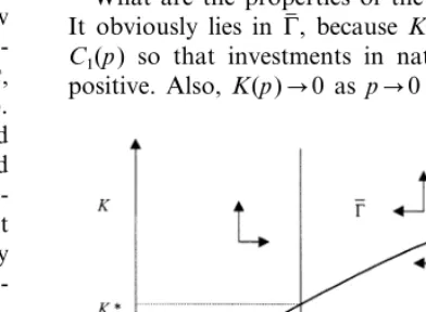
Let g be the curve in (p,K)-space given by
a(p)=R(p,K), see Fig. 1. It divides the space
into two regions. For (p,K) above the curve
(region G) investments are obviously positive. For
values below the curve (regionG) investments are
zero.
Since the initial stock of natural capital is given,
the input price p has to be chosen optimally.
Therefore, the question addressed next is what will happen if the initial values of pare chosen in either of these two regions.
We first consider the positive investment region
G. Take a fixed price p\0. Let
(C1(p), C2(p), y(p)) solve Eqs. (3) and (4) with
r=a(p) inserted. All these functions are well
defined by virtue of the properties of the utility functions and the production functions. It follows from Eq. (4) thatp;/p=0 ifr(p)G1(1/y(p), 1)=r.
Define p* as the (unique) solution of this
equa-tion. Furthermore, it follows from Eqs. (1) and
(2), and the fact that F and H are homogeneous
that K: =0 if
K:=K(p)= C1(p)
G(1, y(p))+
C2(p)
G(1, y(p))F(1, x(p))
What are the properties of the curve (p,K(p))? It obviously lies in G(, because K(p)G(1, y(p))\ C1(p) so that investments in natural capital are
positive. Also, K(p)0 as p0 because if p0
then C1(p)0, C2(p)0, G(1, y(p)) and
F(1, x(p)) . We conclude that there exists a stationary point in G(, denoted by (p*,K*).
In Fig. 1 the arrows indicate the directions in
whichKandpgo from any point inG(. Obviously
K: \0 if and only ifK\K(p). Hence, the picture
strongly suggests that for any K0BK*, one can
find p(0) such that (p(0), K0) lies in G( and such
that the resulting path converges to (p*,K*), This is indeed the case, as is shown in the first theorem.
Theorem 1. Let (C1,C2,K,I,V,W) constitute an
optimal trajectory. Suppose K0BK*. Then
(i) (p(t), K(t))G( for all t.
(ii) (p(t), K(t))(p*,K*) as t , where con -6ergence is monotonic.
(iii) The rates of consumption monotonically
decrease.
(iv) I(t)\0 and W(t)\0 for all t.
Proof 1. The proof of the first two statements is
given in the Appendix A. The proof of (iii)
fol-lows immediately from the fact that p is
increas-ing. The final statement follows from (i).
The theorem essentially states the following. If the initial stock of natural capital is sufficiently small then in a utilitarian optimum there will always be investments to manage natural capital in a proper way. Moreover, natural capital monotonically increases to a steady state and rates of consumption decrease monotonically, also to positive steady states. It is interesting to perform a sensitivity analysis with respect to the rate of time preference. Clearly the steady statep
decreases as r increases. Therefore, a larger rate
of time preference reduces the steady-state rates of consumption, as well as the steady-state stock of natural capital. This conforms with intuition.
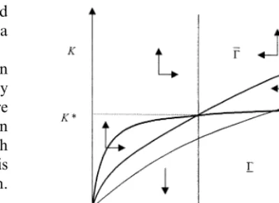
The case K0\K* is less straightforward to
analyse. The proof of Theorem 1 uses the exis-tence of a so-called stable branch in the region G(
defined for all (p,K)5(p*,K*). This branch is a curve inG(, denoted by, K (p), having the property that it is followed along an optimal trajectory
K(t)=K (p(t)). The curveK (p) is also defined for
p\p* but it might be the case that the curve
Fig. 2. Phase diagram forK0\K*.
intersects the curve g and hence lies in G for p
sufficiently large. This, for example, occurs if the elasticities of marginal utility (denoted by h1 and
h2) are constant and satisfy 1\h2\h1. For a
proof of this assertion the reader is referred to the appendix. In this example, which is depicted in Fig. 2 below,K (p) intersectsgonly once, say, but it cannot be excluded that there is more than one point of intersection. However, that is not rele-vant for the main purpose of the present paper,
namely, to show that also for K0\K*
invest-ments in natural capital are positive from some moment in time on.
The optimum is characterised in the following theorem.
Theorem 2. Let (C1,C2,K,I,V,W) constitute an
optimal trajectory. Suppose K0\K*. Then
(i) (p(t), K(t))G( for all t]t0 for some t0]0.
(ii) (p(t), K(t))(p*,K*) as t , where con -6ergence is monotonic.
(iii) The rates of consumption monotonically
decrease.
(iv) I(t)\0 and W(t)\0 for all t]t0.
Proof 2. Parts (i) and (ii) are proven in the
Appendix A. Parts (iii) and (iv) follow immedi-ately from (i) and (ii).
will be no investments directed towards the man-agement of natural capital. But eventually natural capital will approach a positive steady state. Along the approach path near the steady state there will be positive investments. Investments are also positive in the steady state and are just enough to keep natural capital intact given the rate of exploitation. The rates of consumption are high initially but they will decrease to a positive steady state level.
4. Conclusions
We have given a characterisation of the opti-mal use of natural capital in a model with a utilitarian objective. The main outcome is that in spite of a positive rate of time preference natural capital will not vanish; on the contrary, it converges to a positive steady state. If the initial stock of natural capital is small, the stock will increase over time. Also the use of capital will increase, accompanied by increasing invest-ments in natural capital. If natural capital is ‘very large’ initially, it is optimal not to invest in natural capital initially. But from some mo-ment in time on this is no longer the case. Fi-nally, with the rate of time preference tending to zero the steady state stock of natural capital tends to infinity. These statements are not meant to be reassuring because there is the well-known decentralisation problem. Furthermore, perhaps our production functions allow for more substi-tution than is actually warranted. It is our con-jecture, however, that the qualitative results will not drastically change. The idea behind this in-tuition can be sketched as follows. Suppose that there is strict complementarity between natural
capital and labour in the production function G.
Then this can be captured mathematically by
replacing V by K everywhere, also in the
objec-tive function. However, that does not change the problem in any essential respect. It will turn out again that convergence to a steady state will occur. However, the crucial assumption of the paper is that natural capital can be increased through human activities.
Appendix A
In this appendix a proof is given of Theorems 1 and 2 and of the assertion that with constant elasticities of marginal utility it is optimal to have no investments in natural capital initially if the
initial endowment is large. Recall that xW/I
and yV/K. For x\0 we have
r=F1(x, 1); p=F2(1,x)
F(1,x)=a(p)−a%(p)p
The first two equalities follow from the necessary condition (Eq. (5)). The third one follows from
the homogeneity of F.
Lemma A1. Let (p(t), K(t)) be a cur6e satisfying
the necessary conditions (Eqs. (1) – (5)) and let
(p(t), K(t))G( for all t]t0 for some t0]0. Then
(p(t),K(t))(p*,K*) as t .
Proof A1.If(p,K)G( thenr=a(p) and henceyis
a function ofp only (see (Eq. (4)). Therefore, Eq. (5) is an autonomous differential equation with
p(t)p* as t . Define C1(t)C1(p(t)),
C2(t)C2(p(t)), g(t)G(1,y(p(t))) and
f(t)F(1,x(p(t))). So, omitting the argument t
when there is no danger of confusion, we have
K: =IF(1,W/I)−C2
=(KG(1,V/K)−C1)F(1,W/I)−C2
=g(t)f(t)K−C1(t)f(t)−C2(t)
Hence, for t]t0
K(t)=e
&
t
t0
g(t)f(t) dt
!
K(t0)−
&
t
t0
e
−
&
s
t0
g(t)f(t) dt(C
1(s)f(s)+C2(s)) ds
"
The expression between brackets is monotonically decreasing and nonnegative. It converges to a
limit D]0. Suppose D\0. We have
p;/p=F1(1/x(p), 1)G1(1/y(p), 1)−r
Sincep;/p0 ast , it follows thatF1G1ras
t . Then the homogeneity of the functions
implies that there exists t(\t0 ando\0 such that
K(t)\De
&
C2 are bounded because p is bounded. Therefore
e−rtK(t) ast cannot be optimal. This is
a contradiction. So, D=0, and
lim
1. We proceed in several steps 1.1. for0BpBp*
is a decreasing function of p. Therefore,
The combination of the two previous lemmata yields Theorem 1. Next we deal with the case of constant elasticities of marginal utility (h1andh2)
and show that the stable branch does not lie inG(
entirely.
Lemma A3. Suppose 1\h1\h2\0. Then there
exists p\p* such that (p, K(p))g.
Proof A3.It follows from Eqs. (3) and (4) that
−h1
To prove Theorem 2 we proceed as follows. In
GI=W=0. Now define C01(K), Y0 (K), r˜(p,K) as
the solution of C1=KG(1,y), U%1(C1)=r/p,
G2(1,y)=6p/r. It is easily verified that C01 and y˜
depend onKonly. MoreoverC01is increasing and
y˜ is decreasing, so that
p;/p=rG1(K,V)−r
=pU%(C0 1(K))G1(1/y˜(K), 1)−r
is decreasing in K (in G). Now consider the
fol-lowing system of differential equations
K: = −C2(p)
p;
p=pU%1(C01(K))G1(1/y˜(K), 1)−r
Obviously K is decreasing. p;=0 if and only if
References
Ayres, R., 1997. Comments on Georgescu-Roegen. Ecol. Econ. 22, 285 – 287.
Ayres, R., 1998. Eco-thermodynamics: economics and the second law. Ecol. Econ. 26, 189 – 209.
Baum, R., 1976. Existence theorems for Lagrange control problems with unbounded time domain. J. Optim. Theory Appl. 19, 89 – 116.
Clark, C., 1997. Renewable resources and economic growth. Ecol. Econ. 22, 275 – 276.
Daly, H., 1997a. Georgescu-Roegen versus Solow/Stiglitz. Ecol. Econ. 22, 261 – 266.
Daly, H., 1997b. Reply to Solow/Stiglitz. Ecol. Econ. 22, 271 – 273.
Dasgupta, P., Heal, G., 1974. The optimal depletion of ex-haustible resources. Rev. Econ. Stud. Symp. Exex-haustible Res. 14, 3 – 28.
Dasgupta, P., Heal, G., 1979. Economic Theory and Ex-haustible Resources. James Nisbet and Co, Welwyn. Gerlagh, R., 1999. The Efficient and Sustainable Use of
Envi-ronmental Resource Systems. Thelathesis, Amsterdam. Opschoor, H., 1997. The hope, faith and love of neoclassical
environmental economics. Ecol. Econ. 22, 281 – 283.
Pearce, D., Turner, R., 1990. Economics of Natural Resources and the Environment. Harvester Wheatsheaf, Hertford-shire.
Seierstad, A., Sydsaeter, K., 1987. Optimal Control Theory with Economic Applications. North-Holland, Amsterdam. Solow, R., 1956. A contribution to the theory of economic
growth. Q. J. Econ. 70, 65 – 94.
Solow, R., 1974a. Intergenerational equity and exhaustible resources. Rev. Econ. Stud. Symp. Exhaustible Res. 14, 29 – 45.
Solow, R., 1974b. The economics of resources and the re-sources of economics. Am. Econ. Rev. 64, 1 – 14. Solow, R., 1997. Reply. Georgescu-Roegen versus Solow/
Stiglitz. Ecol. Econ. 22, 267 – 268.
Stiglitz, J., 1974. Growth with exhaustible natural resources: efficient and optimal growth paths. Rev. Econ. Stud. Symp. Exhaustible Res. 14, 123 – 137.
Tisdell, C., 1997. Capital/natural resource substitution: the debate of Georgescu-Roegen (through Daly) with Solow/ Stiglitz. Ecol. Econ. 22, 289 – 291.
Toman, M., 1985. Optimal control with an unbounded hori-zon. J. Econ. Dyn. Control 9, 291 – 316.
Weitzman, M., 1998. The Noah’s ark problem. Econometrica 99, 1279 – 1298.