MEASUREMENT ERROR WITH DIFFERENT COMPUTER VISION TECHNIQUES
O. Icasio-Hern´andeza,b∗, Y. I. Curiel-Razob, C. C. Almaraz-Cabralb, S. R. Rojas-Ramirezb, J.J. Gonz´alez-Barbosab aCentro Nacional de Metrolog´ıa, km. 4.5 carretera a los Cu´es, el Marqu´es, Qro., M´exico. - [email protected]
b
Instituto Polit´ecnico Nacional (CICATA), Cerro Blanco No. 141, Colinas del Cimatario Qro., M´exico. -(yajaira.curielrazo, cesarcruzalmaraz, gonzbarjj)@gmail.com, [email protected].
KEY WORDS:Estimation error, Image reconstruction, Measurement techniques, Measurement uncertainty
ABSTRACT:
The goal of this work is to offer a comparative of measurement error for different computer vision techniques for 3D reconstruction and allow a metrological discrimination based on our evaluation results. The present work implements four 3D reconstruction techniques: passive stereoscopy, active stereoscopy, shape from contour and fringe profilometry to find the measurement error and its uncertainty using different gauges. We measured several dimensional and geometric known standards. We compared the results for the techniques, average errors, standard deviations, and uncertainties obtaining a guide to identify the tolerances that each technique can achieve and choose the best.
1. INTRODUCTION
Several imaging techniques for accurate 3D reconstruction and their quality is improving rapidly. Some authors like (Hocken, 2011), (Maier-Hein, 2013), (Rashmita, 2013) and (Ng, 2011) be-lieve that an evaluation is necessary for these techniques, so they assess the process algorithms to determine the quality of the mea-surements.
The purpose of this work is to assess the measurement error of passive stereoscopy, active stereoscopy, shape from contour and fringe profilometry using different known dimensional gauges. The techniques considered apply algorithms to fit a set of points from a gauge image to a particular geometry. The gauge measure-ment error define the quality of the technique. Authors as (Rash-mita, 2013), (Ng, 2011) and (Salvi, 2007) suggest that industry can use these techniques for quality control if the measurement error and its uncertainty is under the verified tolerances.
The gauge measurement error is defined as the measure calcu-lated with the technique minus the known value of the gauge. The nominal used lengths were 3mm, 50mmand 100mmblock gauges, a 10mmmetallic pin diameter, and a height of 15.081 mmof fine-grained 3D printed piece of gypsum, see Figure 1.
Figure 1. Gauges used to measure the error of different optical measurement techniques.
The closest work to our own investigations has been proposed by (Ramos,2011), who instead of implemented techniques used dif-ferent instruments with digitization techniques incorporated into
∗Corresponding author
its measurement software and similar to our work he used dif-ferent reference gauges. Most of the reported vision techniques in (Hocken, 2011), (Maier-Hein, 2013), (Rashmita, 2013), (Ng, 2011) and (Salvi, 2007) offer measurement errors using objects with no traceability. Our work report measurement errors using gauges with traceability to national standards.
This paper is organized as follows. Section 2 deals with the un-certainty applied to the results. In section 3, we implemented the 3D reconstruction techniques including references, calibra-tion process, the particular experimental setup and the results. The comparative results between techniques are given in section 4 and section 5 deals with the conclusions and discussion about results.
2. UNCERTAINTY
2.1 Uncertainty applied on results
In accordance with (ISO 14253-1, 1998) every measurement pro-cess must take into account the accuracy (ISO 14253-1, 1198) represented by a resultant error and its corresponding uncertainty. We based the uncertainty calculation on the guide to the ex-pression of uncertainty in measurement (GUM, 2010) and (ISO 15530-3, 2011) Coordinate Measuring Machines (CMM): Tech-nique for determining the uncertainty of measurement Part 3: Use of calibrated work pieces or measurement standards (ISO 15530-10, 2011). The expanded uncertainty expression U for our error measurand is:
U =k·uc(y) =k·
p
u2
cal+u2p+u2b+u2w (1)
wherekis the coverage factor with a conventional value of two to achieve a probability of 94.5% of confidence in the calculated uncertainty.uc(y)is the combined uncertainty of each
contribu-tory. ucalis the standard calibration uncertainty reported in the
certificate of calibration of the gauge reference used. upis the
speed of measurement, and geometry of the measuring system. ubis the standard uncertainty associated with the systematic
er-rorbof the measurement process evaluated using the calibrated work piece, in our case the systematic error is the measurand so ubwill not be considered. uw, is the standard uncertainty of the
material and the variations of manufacture, it includes sources of uncertainty as variations in thermal expansion, errors of shape, roughness, elasticity, and plasticity.
Due to the error ranges of the implemented techniques and the quality of the gauges ucal, ub anduw are considered zero so
Equation 1 is simplified as follows:
U =k·pu2
p (2)
From Equation 2, the uncertaintyupis Equation3:
up= σ x
√
n (3)
whereσxthe standard deviation of the measurements defined in
Equation4, andnis the number of measurements.
σx=
r
Σn
j=1(qj−q¯)2
n−1 ; (4)
wherenis the number of measurements,qjis thejmeasurement
andq¯is the mean of the measurements.
All the techniques were implemented in a laboratory with a tem-perature of20o±3oC, with artificial illumination and the
ab-sence of direct sunlight. The number of measurements made with each technique is at leastn= 3to calculate uncertainty. The un-certainties of calibration certificate for the gauges used are in the range of±12nmto±250nmwhich, as mention before, were consider as approximately zero for the case of the implemented techniques.
3. 3D RECONSTRUCTION TECHNIQUES
3.1 Passive Stereoscopy Technique (PST)
According with (Szeliski, 2010), in computer vision, the topic of Passive Stereoscopy Technique (PST), specially stereo match-ing, has been one of the most widely studied and fundamental problems, and continues to be one of the most active research areas. While photogrammetric matching concentrated mainly on aerial imagery, computer vision applications include model-ing the human visual system, robotic navigation and manipula-tion, as well as view interpolation and image-based rendering, 3D model building, and mixing live action with computer-generated imagery.
3.1.1 Calibration method and model for PST To calibrate the cameras we considered the model proposed by (Hall, 1982) and (Tsai, 1987) both uses the pinhole camera model. This model is extended with some correction parameters, such as radial lens distortion and tangential lens distortions that causes radial and tangential displacement in the image plane.
Camera calibration means the process of determining the internal camera geometric and optical characteristics (intrinsic parame-ters) and/or the 3D position and orientation of the camera frame
relative to a certain world coordinate system (extrinsic parame-ters). The purpose of the calibration is to set a relationship be-tween 3D points from the world and 2D points from the image, seen by the computer (Tsai, 1987), (Heikkila, 1997), and (Vilaca, 2010).
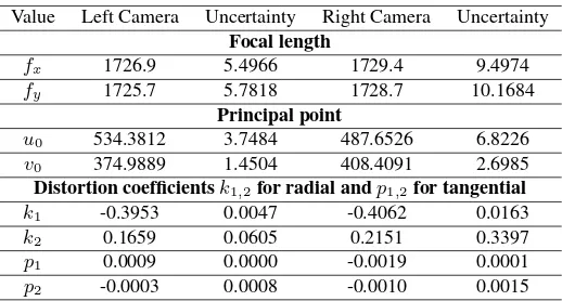
We performed cameras calibration for PST with the toolbox from (Bouguet, 2013) that uses a checkerboard calibration pattern. Ta-ble 1 shows the results of the intrinsic parameters for each camera and its uncertainties.
Table 1. Camera calibration results for Passive and Active Stereoscopy Techniques.
Value Left Camera Uncertainty Right Camera Uncertainty Focal length
fx 1726.9 5.4966 1729.4 9.4974
fy 1725.7 5.7818 1728.7 10.1684
Principal point
u0 534.3812 3.7484 487.6526 6.8226
v0 374.9889 1.4504 408.4091 2.6985
Distortion coefficientsk1,2for radial andp1,2for tangential
k1 -0.3953 0.0047 -0.4062 0.0163
k2 0.1659 0.0605 0.2151 0.3397
p1 0.0009 0.0000 -0.0019 0.0001
p2 -0.0003 0.0008 -0.0010 0.0015
3.1.2 PST experimental setup The cameras used in this technique were two AVT Marlin F-145C 2 with IEEE 1394 IIDC FireWire interface with a resolution of 1280 x 960 pixels, and a laser beam to project a dot pattern, not necessary in this tech-nique; however, for simplicity this work decided to use the laser to detect correspondence points between cameras as quick as pos-sible.
Figure 2(a) shows the setup with 2 cameras at approximately an angle of29o
between the optical axis of the cameras and the bar that holds the set up, and a laser that projects a point pattern over the measured gauge. Figure 2(b) shows the target point at the central part of the gauge block and the points on the origin plane. Figure 2(c) displays the correspondence points projected onto gauges and observed with both cameras. The matching of the points for each image of the left and right cameras generates an arrangement of points that represents the height of the gauge blocks and the height of the pyramid between the first level and the top level.
The resulting 3D reconstruction depends on image quality. In order to obtain images of sufficient quality we acquired experi-mental images under good illumination conditions as mentioned in (Belhaoua, 2010) and (Muquit, 2006).
We fitted a planeπ :ax+by+cz+d= 0and a pointp1 =
(x1, y1, z1)outside the plane to calculate the measurements. The
shortest distance fromp1to plane is defined in Equation5:
D=|ax1√+by1+cz1+d|
a2+b2+c2 (5)
where a, b, c and d are the coefficients of the plane and
(x1, y1, z1)represents a point outside the plane.
(a) Stereoscopy system.
(b) 3D Points(mm).
(c)Dots projection over a gauge block of 50mm.
Figure 2. Passive stereoscopy setup.
of gypsum (Pyramid). Based on (Hocken, 2011), the main factors influencing the accuracy of a stereovision system are as follows: defects of optical systems, errors caused by image processing, quality of the target, arrangement of the cameras, calibration er-rors, thermal error and stability camera mounting. The reported errors in Table 2 occurred due to different factors:
• Manual selection of correspondence points detected in both cameras, see Figure 2.
• The quality projection of the points is low.
• The angle arrangement of the cameras to the normal of the plane is less than45o.
Table 2. Results of Passive Stereoscopy Technique.
Value (mm) Block 3 Block 50 Block 100 Pyramid 15 True value 3.000 50.000 100.000 15.081
Average 2.848 47.776 91.846 13.455
Error -0.152 -2.224 -8.154 -1.626
σ 0.208 3.451 0.501 0.474
Uk= 2 0.186 3.086 0.448 0.424
The technique shows measurement errors greater than 2 mm when measured dimension exceeds 50mmwhich is higher than the reported in the literature (Belhaoua, 2010). As a result, this technique seems to be unsatisfactory for measuring dimensions over 50mm. Table 2 shows that the increasing size of the gauge is directly proportional to the average error.
3.2 Active Stereoscopic Technique (AST).
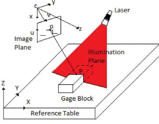
One of the most popular active illumination devices is a laser or light stripe, which sweeps a plane of light across the scene or object while observing it from an offset viewpoint (Rioux, 1993) and (Curless, 1996), see Figure 3.
Figure 3. Illumination plane for 3D reconstruction with active stereoscopy.
The laser and the offset viewpoint (commonly a camera) en-close the Active Stereoscopic Technique (AST). As the stripe falls across the object, it deforms according to the shape of the surface it is illuminating. Then using optical triangulation we es-timate the 3D locations of all the points seen in a particular stripe. In more detail, knowledge of the 3D plane equation of the light stripe allows us to infer the 3D location corresponding to each illuminated pixel. The accuracy of light striping techniques im-proves by finding the exact temporal peak in illumination for each pixel (Curless, 1996).
3.2.1 Calibration method and model for AST As in PST, the employed model is the pinhole, just the way to calculate ex-trinsic parameters is different. Table 1 shows right camera intrin-sic parameters and its uncertainties. For this method is necessary to obtain the equation of the line-plane from the laser beam de-picted in Figure 3. This work used four heights: 3mm, 50mm, and 100mmgauge blocks, and the reference plane. We fit four points from the top of these gauge blocks and 400 points from the reference plane outside the gauge blocks, giving a total of 404 points used to determine the plane of the line.
3.2.2 AST experimental setup Figure 4(a) shows the setup used on this technique. This setup was extracted from the PST setup depicted in Figure 2(a) using only the right camera and the laser.
In total, fifteen planes must be found equivalent to firteen lines according to the pattern of light generated by the laser (see Figure 4(a)). However we only need to find the plane equation of the line that the experimental setup from Figure 4(a) allows passing.
This plane will lead to the dimensional reconstruction of gauges blocks, and allows the determination of the depth of the object from the camera, see Figure 3.
3.2.3 Results of AST We used 3mm, 50mmand 100mm length gauge blocks to test AST. Table 3 shows results calculated using fitted lines adjusted to the reference plane and a maximum point found on the peak of the signal see Figure 5.
(a) Experimental setup for Ac-tive Stereoscopy.
(b) Online 3D reconstruction of some mea-sured gauges.
Figure 4. Active Stereoscopic Technique setup and measurement.
Table 3. Results of active stereoscopy technique.
Value (mm) Block3 mm Block 50 mm Block 100 mm
True value 3.000 50.000 100.000
Average 3.537 50.232 101.848
Error 0.537 0.232 1.848
σ 0.021 0.007 0.004
Uk= 2 0.019 0.006 0.003
procedure we used the same printed pattern like in PST, but AST only use the right camera, which according to Table 2 does not have the same left camera intrinsic parameters (focal length, prin-cipal point and distortion). The highest standard deviation ac-cording to Table 3 is 0.021mm; this was due to the thickness of the light used. It generates noise that affects the image pro-cessing of pieces with dimensions less than 3mm, see Figure 5. Furthermore, the surface material where the light beam is pro-jected is a factor that contributes to noise. Table 3 also shows the average error for the 50mmand 100mmgauges blocks in-creases from 0.232mmto 1.848mmproportional to its size, it is proposed to use a correction factor (usually linear) that change with the dimensions of the piece to be measured. This technique consists on a triangulation principle between the laser transmit-ter, the measured point and the camera. (Hocken, 2011) men-tioned that the measured results of this technique depend heav-ily on the structure and angle of inclination of the surface (see Figure 3). This leads to relatively large measuring uncertainties making the use of this technique suitable only for less demanding applications. (Hocken, 2011) mentioned that better results can
(a) 3mmgauge block measure.
(b) 50mmgauge block measure.
Figure 5. 2D reconstructions of gauge blocks using AST.
be achieved with laser sensors working according to the Focault principle.
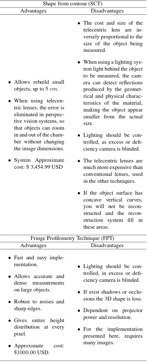
3.3 Shape from Contour Technique (SCT)
(Baumgart, 1974) introduced the idea of using contours for 3D reconstruction. Afterwards (Szeliski, 1993) proposed a non-invasive digitizer built using a rotary table and a single cam-era with the reconstruction procedure of Shape from Silhouette (SFS) or Shape from Contour (SFC). SFS has become one of the most popular methods for the reconstruction of static objects (Gonzalez-Barbosa, 2015), (Fitzgibbon, 1998) and (Fang, 2003). SFC presents results with errors for objects of high complexity or detailed (Rodr´ıguez, 2008).
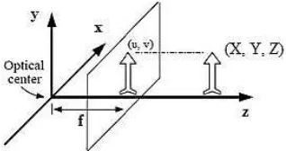
3.3.1 Calibration method and model for SCT We based on (Gonzalez-Barbosa, 2015). The orthographic geometry il-lustrated in Figure 6, is the projection of a three dimensional pointQ(X, Y, Z)over a plane image generates a pointq(u, v)
.Whereu =X andv =Y. Then, the model Equation 6 of or-thographic projection in homogeneous coordinates[u, v,1]Tof a
point[X, Y, Z,1]T
is
q=KEQ (6)
whereKis defined as the matrix of intrinsic parameters, andE as the matrix of extrinsic parameters, see Equation7
K=
α γ 0 0
0 β 0 0 0 0 0 0
!
;E=
R T
0 1
(7)
The elements ofKinclude: αandβ, the scale factors in image uandvaxes, andγthe parameter describing the skewness of the two image axes. The matrixErepresents the rigid transformation that carries the world coordinate system to the image coordinate system, composed of a rotationR∈ R3x3 and a translationT ∈R3.
Figure 6. Orthographic projection model of a real object into the image plane.
K=
14.325 0 0 0 0 15.533 0 0 0 0 0 1
!
The Equation used to convert the data from 2D image coordinates to 3D world coordinates is defined by:
Q=E(−1)K(−1)q (8)
whereQis a3x1vector representing 3D world coordinates and qis a3x1vector of each pixel from the subpixelic contour. The Shape reconstruction From the contour technique was tested us-ing 3mm, 50mmgauge blocks and the 10mmcylinder gauge.
3.3.2 SCT experimental setup The SFC system used a tele-centric lens (OPE TC 1364 by Opto Engineering), a turntable with a high accuracy encoder and 2.16 arc sec resolution (CR1-Z7 by Thorlabs), and calibration pattern (PT 036-0596 by Opto Engineering), depicted in Figure 7.
Figure 7. Shape from Contour setup.
Images of a rotating object illuminated from its back side are ren-dering. Consequently, the acquisition system can only see the contour of the object, as shown in Figure 8. We took 73 images with 5 degrees steps,i= 0,5, . . . ,360.
Figure 8. Cylinder images acquisition.
After the image acquisition, we applied a sub pixel extractor. The angle of rotation was calculated as the product of the image index with the rotation angle indicated by the turntable.
Using only one axis of rotation in all the images leads to inaccu-rate results. This inaccuracy is due to slight changes of the axis of rotation coming from illumination fluctuations and misalignment of the work piece with respect to the rotation of the turntable and the position of the camera. A dynamic rotation axis is neces-sary to reduce this inaccuracy. The first degree polynomial is a straight line fitted to all points over the subpixel contour image. This Equation is of the form:
Au+Bv+C= 0 (9)
whereu and vare pixel coordinates andA, B, C are the line coefficients.
Once calculated the dynamic axis of rotation, we have to perform a translation and rotation (eccentricity and leveling of the work piece with respect to the camera) of the coordinate system in pixel coordinates to the dynamic axis of rotation. This axis of rotation allows the 3D reconstruction with the accuracy showed in Table 4.
Table 4. Results of Shape from Contour Technique.
Value (mm) Block 3 mm Block 50 mm Cylinder 10 mm
True value 3.000 50.000 10.000
Average 2.924 49.887 9.785
Error -0.076 -0.113 -0.215
σ 0.007 0.006 0.040
Uk= 2 0.008 0.007 0.046
At the same time, each one of the contour sub-pixel images was rotated around the X axis, and the gauge was plotted to show in real time the 3D reconstruction of the gauge, see Figure 9. Finally, the pixel coordinates were transformed to world coordi-nates using Equation 8.
Figure 9. 3D reconstruction of 10mmcylinder gauge.
3.3.3 Results of SCT In this technique we measured gauges three times. The measurement system acquired 73 images ev-ery5o
degrees in360o
the technique provided better repeatability and lower uncertainty than AST and PST.
3.4 Fringe Profilometry Technique (FPT)
This technique for 3D reconstruction uses fringe projection. Ex-ist several algorithms for processing the acquired images and un-wrapping the phase, such as Fourier profilometry, phase shifting profilometry and temporal unwrapping profilometry technique, these are mentioned in (Rodriguez, 2008), (Takeda, 1983), (Villa, 2012) and (Cogravve, 1999).
We choose the temporal unwrapping profilometry technique tested in (Huntley, 1997) and (Xiao, 2010) because it is immune to noise and big gradients in test objects. It consists on projecting fringes with different periods at shifted phase; in our work we use, four imagesIishifted 90 degrees att= 1,2, . . . ,7different
frequencies.
The wrapped phase map for the value oft= 1is calculated with the Equation 10 for phase shifting.
φw(t) =tan−1
I4−I2
I1−I3
(10)
For the next phase maps, we use the Equation 11
∆Φw(i, j) = arctan
∆I42(t)∆I13(j)−∆I13(t)∆I42(j)
∆I13(t)∆I13(j) + ∆I42(t)∆I42(j)
(11)
where
∆Ikl(t) =I(k, t)−I(l, t) (12)
Finally, to find the unwrapped phase U, we apply the recursive equation with two consecutive wrapped phase maps. Equation 13
U[Φ1,Φ2] = Φ1−2πN IN T
Φ1−Φ2
2π
(13)
With the value of the unwrapped phase, we can perform the cali-bration to calculate the metric values of the test object.
3.4.1 FPT calibration We performed the system calibration in two stages according to (Villa, 2012), the first one is the axial calibration which consisted in take 5 planes inZ axis direction with known increments∆Z (in this case 10mm). We project fringes according to (Cogravve, 1999) and (Huntley, 1997) on ev-ery plane and calculate a4th
degree polynomial regression with the phase values in every plane at the knownZpositions.
Once we have this relationship, we proceed with axial calibration, to this we used a grid pattern with a 2cmperiod and a bright dot in the point that we assume as the origin, see Figure 10. When the calibration is finished, we put the calibration gauges on the reference plane, and project fringes as showed at Figure 11.
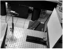
3.4.2 FPT experimental setup. The experimental set up con-sisted of a Marlin F-080 CCD camera, a digital projector SONY VPL-EX5, both1024x768pixels resolution, a flat surface and a millimetric rail shown in Figure 12.
Figure 10. Grid pattern with 2cmperiod.
Figure 11. One of the acquired images.
3.4.3 Results of FPT Pyramid and calibration gauges recon-struction is showed at Figure 13 and 14.
Table 5 shows standard deviations less than 0.107mm which demonstrate repeatability of the instrument. The average error increases with the time of use (about one hour) due to projector heating.
4. COMPARATIVE RESULTS BETWEEN TECHNIQUES
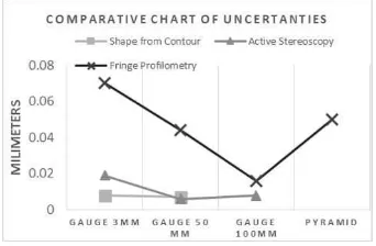
Figure 15 shows the measurement error of different gauges for the implemented technique. SFC has the best accuracy compared with the other three implemented techniques.
As shown in Figure 15, the average error in PST, AST and FP grows according to the size of the gauge because the viewing an-gle of the camera changes with the height of the measured piece; this suggests a correction of the measuring points with respect to the reference surface.
Figure 16 shows the uncertainties of the implemented techniques. In this Figure we can see that AST, SFC and FP are comparable, in these measurement systems the uncertainty decreases when the size of the piece is increasing. These systems show low repeata-bility to reconstruct pieces less than 3 mmin size. SFC also reduces uncertainty by increasing the size of the piece, without breaking its measurement range.
Figure 13. 3D reconstruction of pyramid, axis are at centimeters.
100 mm block
50 mm block
3 mm block
Figure 14. 3D reconstruction of the blocks, axis are at centimeters.
Uncertainties values of PST are out of scale with respect to the values of the other techniques in Figure 16.
5. CONCLUSIONS AND DISCUSSIONS
According with (Hocken, 2011) all of the implemented tech-niques can be improved in the calibration process if consider: image processing algorithms, temperature, intensity of illumina-tion, optical magnificaillumina-tion, imaging optics, telecentricity, camera resolution, edge detection technique, material of reference, refer-ence surface tilt, optical magnification of laser sensor, scanning speed and laser intensity.
The software used to fit the points captured by any of the imple-mented techniques have a greatly influence on the quality of the measured results. We recommend use software with a calibration certificate. SFC, AST and PF, average errors, standard deviations, and uncertainties obtained with the present approach can help the user to identify the tolerances that each technique can achieve and to determine if these techniques can be applied to the control of some quality process or measuring process.
The performance of PST shows poor results for the tolerances that were expected based on (Belhaoua, 2010). Because of this, it is bad for quality control purposes, unless improvements in the factors considered on results of PST are done. Tables 6 and 7 de-scribe the advantages and disadvantages of each technique. These
Table 5. Results of Fringe Profilometry Technique.
Value (mm) Block 3 Block 50 Block 100 Pyramid 15 True value 3.000 50.000 100.000 15.081
Average 2.848 51.919 102.913 14.315
Error -0.152 1.919 2.913 -0.766
σ 0.098 0.088 0.028 0.107
Uk= 2 0.070 0.044 0.016 0.050
Figure 15. Comparative chart for average errors. X-axis shows the measured objects and Y-axis the average error inmm.
Figure 16. Comparative chart for uncertainties. X-axis shows the measured objects and Y-axis the uncertainties atmm.
tables let the user to take a decision. For example we can say that PST can be used on computer vision implementations, like robot navigation, but SFC, AST and FP can be used on metrological issues, like reverse engineering.
To calibrate the cameras in PST, AST and FP techniques, we used a printed pattern, this implies an error in the calibration results which affects the error of measurement. The printed patterns in-troduce an error that can be considered systematic according to (Xiao, 210) and therefore corrected, however, the residuals once the correction is applied, must be part of the uncertainty measure-ment.
Also the calibration process must take into consideration factors such as temperature of the structure holding the cameras, flatness where the printed pattern are pasted, humidity, image processing and others. These and other errors can have a systematic nature and can be corrected, improving the measurement error. These corrections influence the error measurement uncertainty .
The method used by the SFC technique is very different from PST, AST and FP techniques where a pinhole model is consid-ered. The model used was based on (Gonzalez-Barbosa, 2015); however, we must consider that the model could have other errors not considered like the heating of the screen light from Figure 7. In its favor, this technique uses a certificate pattern instead of a printed one.
Future work will consider the influence of the above errors for smaller measurement error and find major factors of uncertainty affecting the measurements.
ACKNOWLEDGMENT
Table 6. Reconstruction techniques PST and AST with advantages and disadvantages of our implemented systems.
Passive Stereoscopy Technique (PST)
Advantages Disadvantages
• Can be set to objects of different sizes at different distances in various environmental conditions.
• Did not has correspon-dence problems when a dot pattern was pro-jected onto the sur-face, these projected points simplified the calculation of its 3D position.
• Approximate cost:
$1,101.98USD.
• In the absence of a pro-jection pattern; a point in the image of one of the cameras can be associated with several points on the image of the other camera (false match)
• If exits a hide point by occlusions in the field of view of one cameras maybe in the other field of view of the second camera this point are visible.
• The selection of corre-spondence points was made manually can cause mismatches errors.
Active Stereoscopy (AST)
Advantages Disadvantages
• Currently used in sev-eral commercial
mea-• To establish the re-lationship between the 2D image points and points in the 3D world, the tri-angulation method used.
• Approximate cost:
$1,689.99USD.
• One of the main limita-tions of this technique is the problem of occlusion, which occurs when the camera is not able to dis-play the laser beam re-flected by the object, since the object geometry.
• The camera reaches de-tect unwanted reflections generated by the geomet-ric and physical character-istics of the object.
• The reflected laser beam on the object has a thick-ness and this introduces an impression when de-tecting the light beam in the image acquired by the camera.
• The laser power affects the sharpness of this on pur-pose, because if the in-tensity is not enough, the plane of light will not be detected in the image.
371999), Instituto Polit´ecnico Nacional (IPN) particularly at Cen-tro de Investigaci´on en Ciencia Aplicada y Tecnolog´ıa Avanzada Unidad Quer´etaro (CICATA-Qro) for the financial support given, and Centro Nacional de Metrolog´ıa (CENAM) for the facilities
Table 7. Reconstruction techniques SCT and FPT with advantages and disadvantages of our implemented systems.
Shape from contour (SCT)
Advantages Disadvantages
• Allows rebuild small objects, up to 5cm.
• When using telecen-tric lenses, the error is eliminated in perspec-tive vision systems, so that objects can zoom in and out of the cham-ber without changing the image dimensions.
• System Approximate cost:$3,454.99 USD
• The cost and size of the telecentric lens are in-versely proportional to the size of the object being measured.
• When using a lighting sys-tem light behind the object to be measured, the cam-era can detect reflections produced by the geomet-rical and physical charac-teristics of the material, making the object appear smaller from the actual size.
• Lighting should be con-trolled, as excess or defi-ciency camera is blinded.
• The telecentric lenses are much more expensive than conventional lenses, used in the other techniques.
• If the object surface has concave vertical curves, you will not be structed and the recon-struction system fill in these areas.
Fringe Profilometry Technique (FPT)
Advantages Disadvantages
• Fast and easy imple-mentation.
• Allows accurate and dense measurements on large objects.
• Robust to noises and sharp edges.
• Gives entire height distribution at every pixel.
• Approximate cost:
$1000.00USD.
• Lighting should be con-trolled, in excess or defi-ciency camera is blinded.
• If exist shadows or occlu-sions the 3D shape is loss.
• Dependent on projector power and resolution.
• For the implementation presented here, requires many images.
REFERENCES
Baumgart B., 1974. Geometric Modeling for Computer Vision. PhD Thesis, Stanford University.
Belhaoua A., Kohler S. and Hirsch E., 2010. Error Evaluation in a Stereovision-Based 3D Reconstruction System. EURASIP Journal on Image and Video Processing pp. 1-12.
Bouguet, J. Y., 2013. Camera calibration toolbox for MatLab. Last updated December 2ˆnd, 2013.
Bolles R. C., Kremers J. H. and Cain R. A., 1981. A simple sensor to gather three-dimensional data. Technical note 249, SRI.
Coggrave C.R. and Huntley J.M., 1999. High-speed surface pro-filometer based on a spatial light modulator and pipeline image processor. Opt. Eng., 38(9), pp. 1573-81.
Curless B., and Levoy M., 1996. A volumetric method for build-ing complex models from range images. In ACM SIGGRAPH 1996 Conference Proceedings, pp. 303312, New Orleans.
Fang Y. H., Chou H. L. and Chen Z., 2003. 3D shape recovery of complex objects from multiple silhouette images. Pattern Recog-nition Letters, 24(9-10) pp. 12791293.
Fitzgibbon A. W., Cross G. and Zisserman A., 1998. Automatic 3D Model Construction for Turn Table Sequences. In Proceed-ings of the European Workshop on 3D Structure from Multiple Images of Large-Scale Environments, pp. 155-170.
Gonzalez-Barbosa J.J., Rico-Espino J.G., G´omez-Loenzo R.A., Jim´enez-Hern´andez H., Razo M., Gonzalez-Barbosa M, 2015. Accurate 3D Reconstruction using a Turntable-based and Tele-centric Vision. AUTOMATIKA, Vol. 56 (4), pp. 508521.
Evaluation of measurement data - Guide to the expression of un-certainty in measurement, JCGM 100:2008 GUM 1995 with mi-nor corrections. First edition 2008 Corrected version, 2010.
Hall E. L., Tio B. K., JMcPherson C. A. and Sadjadi F. A., 1982. Measuring curved surfaces for robot vision. Comput. Vol. (15), pp. 42-54.
Heikkila J. and Silve O., 1997. A four-step camera calibra-tion procedure with implicit image correccalibra-tion. Proceedings IEEE CVPR, pp. 11061112.
Hocken R. J. and Pereira P. H., 2011. Coordinate Measuring Ma-chines and Systems. 2nd Edition, CRC Press, USA, pp. 30, 129, 131, 134, 135, 149, 493, 494.
Huntley J.M. and Saldner H.O., 1997. Error-reduction methods for shape measurement by temporal phase unwarpping. Opt. Soc. Am.,14(12), pp. 3188-96.
ISO 14253-1, 1998. Geometrical Product Specifications (GPS) Inspection by measurement of work pieces and measuring equip-ment Part 1: Decision rules for proving conformance or non-conformance with specifications, Geneva.
ISO 5725-1/Cor 1, 1998. Geometrical product specifications (GPS) Accuracy (trueness and precision) of measurement meth-ods and results Part 1: General principles and definitions.
ISO 15530-3, 2011. Geometrical product specifications (GPS) Coordinate measuring machines (CMM): Technique for deter-mining the uncertainty of measurement Part 3: Use of calibrated work pieces or measurement standards.
Maier-Hein L., Mountney P., Bartoli A., Elhawary H., Elson D., Groch A., Kolb A., Rodrigues M., Sorger J., Speidel S. and Stoy-anov D., 2013. Optical techniques for 3D surface reconstruction in computer-assisted laparoscopic surgery, Medical Image Anal-ysis, vol. 17, pp. 974996.
Muquit M. A., Shibahara T. and Aoki T., 2006. A High-Accuracy Passive 3D Measurement System Using Phase-Based Image Matching. IEICE TRANS. FUNDAMENTALS, E89A(3).
Ng S. C. and Ismail N., 2011. Reconstruction of the 3D object model: a review, SEGi Review, Vol. 4 (2) pp. 18-30.
Rashmita K., Chitrakala Dr. S. and SelvamParvathy S., 2013. 3D Image Reconstruction: Techniques, Applications and Challenges. Proceedings of International Conference on Optical Imaging Sen-sor and Security, Coimbatore, Tamil Nadu, India.
Ramos B., Santos E., 2011. Comparative Study of Different Dig-itization Techniques and Their Accuracy. Computer Aided De-sign, Vol. 43 (2), pp. 188-206.
Rioux M., and Bird T., 1993. White laser, synced scan. IEEE Computer Graphics and Applications, 13(3), pp. 1517.
Rodr´ıguez J., 2008. T´ecnicas de Reconstrucci´on Volum´etrica a partir de M´ultiples C´amaras: Aplicaci´on en Espacios In-teligentes. Bachelor’s Thesis, Universidad de Alcal´a, Escuela Polit´ecnica Superior, Ingenier´ıa Electr´onica.
Salvi J., Matabosch C., Fofi D. and Forest J., 2007. A review of recent range image registration methods with accuracy evalua-tion. Image and Vision Computing, Vol. 25 (5), pp. 578-596.
Szeliski R., 2010. Computer Vision: Algorithms and Applica-tions. Springer, Chapter 11: Stereo correspondence, pp. 537-567, ISBN: 978-1-84882-935-0.
Szeliski R., 1993. Rapid octree construction from image se-quences. Computer Vision Graphics and Image Processing: Im-age Understanding, Vol. 58(1) pp. 23-32.
Takeda M. and Mutoh K., 1983. Fourier transform profilometry for the automatic measurement of 3-D object shapes. App. Opt., 22(24), pp. 3977-3982.
Tsai R., 1987. A Versatile Camera Calibration Technique for High-Accuracy 3D Machine Vision Metrology Using Off-the-shelf TV Cameras and Lenses. IEEE J. Rob. Autom. Vol. 3(4), pp. 323-44.
Vilaca J. L., Fonseca J. C. and Pinho A. M., 2010. Non-contact 3D acquisition system based on stereo vision and laser triangula-tion. Machine Vision and Applications, Vol. 21, pp. 341350.
Villa J., Araiza M., Alaniz D., Ivanov R. and Ortiz M., 2012. Transformation of phase to(x,y,z)-coordinates for the calibration of a fringe projection profilometer. Opt. Laser Eng., 50(2), pp. 256–261.