DITCH: a model to simulate field conditions in response to ditch levels
managed for environmental aims
Adrian Armstrong
∗ADAS, Gleadthorpe Research Centre, Meden Vale, Mansfield, Notts, NG20 9PF, UK
Received 23 December 1998; received in revised form 9 March 1999; accepted 1 June 1999
Abstract
Wetland areas are frequently managed by manipulating the water levels in the surrounding ditches, with the aim of restoring or enhancing the wetness of the site, especially for the ecological requirements of some bird populations. The extent to which water tables in the centre of fields can be controlled by this action can be simulated through the use of a model, Drain Interaction with Channel Hydrology (DITCH), based on drainage theory. DITCH successfully predicted the pattern of water table behaviour on two wetlands sites, in the Norfolk Broads and Somerset Levels areas in the UK. The model can also be used to predict the strength of the soil surface and the extent of surface flooding. When used to examine the effects of alternative ditch management regimes within the two test areas, the model shows that the effects of ditch management options are not easily converted into impacts in the centre of the fields. If the effects are not sufficient, then hydrological manipulation of sites to achieve or improve wetland status may require more active intervention. ©2000 Elsevier Science B.V. All rights reserved.
Keywords: Wetlands; Water tables; Environmentally sensitive areas; Soil surface strength; Flooding; Hydrology
1. Introduction
Public awareness and concern for the maintenance and preservation of wetlands (Maltby, 1986), has lead to positive action to manage wetland resources. In the past, many wetland areas have been drained, with the aim of increasing agricultural productivity. In an at-tempt to restore wetland status, or to improve the wet-ness of those wetlands that have survived, the same structures that were used to drain the land are now being used to control the wetness, primarily through the control of ditch water levels. These manipulations are intended to improve the ecological status of the
∗Corresponding author. Tel.:+44-1623-844-331; fax:+
44-1623-844-472.
E-mail address: [email protected] (A. Armstrong).
area, as to improve the landscape value. Populations of birds, which are often taken as critical environmental indicator, require soft, wet soils, for feeding; and par-tially flooded areas for breeding. (Tickner and Evans, 1991).
Consequently, governments have introduced agri-environment schemes, in which they encourage (often through payments) the management of agri-cultural areas in environmentally sensitive ways. One such scheme in the UK is the Environmentally Sen-sitive Areas (ESA) scheme, in which the Ministry of Agriculture Fisheries and Food enters into agreements with farmers to adopt practices which seek to con-serve and enhance areas of high landscape or historic value which are vulnerable to changes in agricultural practices. Where the ESAs encompass wetland ar-eas, the agreements may prescribe the water levels in
the ditches, and the land owners have to meet these targets in order to qualify for the relevant payments.
Within such schemes, the practical issue of deter-mining the correct management options (as defined in the terms of the ESA agreements), particularly the ditch water levels that are appropriate, may be subject to debate. As a tool for understanding some of the possible outcomes of adopting specific ditch manage-ment regimes within wetlands ESAs, a model, called DITCH (Drain Intraction with Channel Hydrology) has been developed to examine the consequences of various ditch management regimes (Armstrong, 1993; Armstrong et al., 1993). This paper describes the model, its development and its validation against data sets collected from two sites in the UK, in the Broads ESA and in the Somerset Levels and Moors ESA. The results have been used to indicate the effectiveness of the ESA prescriptions in meeting their ecological and landscape objectives.
2. Model development
To simulate the soil water regime within a field, a model is required to calculate the sequence of water levels in the field in response to the meteorological inputs and the imposed boundary (ditch) conditions. The theory of water movement to drains, derived from an understanding of the physics of soil water flow pro-cesses, is based on Darcy’s Law for saturated flow, leading to the development of a theory of drainage sys-tems that can be used for this study (e.g., Van Schilf-gaarde, 1974; Smedema and Rycroft, 1983; Ritzema, 1994).
The DITCH model is based on the calculation of the water balance in the field, using the fluxes of water moving through the soil to the peripheral ditches, to estimate the changing position of the water table in the field. The water elevation in the field on day t is Mt is, thus, given by:
Mt =
Mt−1+(R−ET−Qd)
f (1)
where R is the rainfall, ET is evapotranspiration, Qd is the discharge through the drainage systems and f is the relevant porosity. For geometrically regular situa-tions such as a uniform soil drained by parallel ditches, the drainage can be calculated from one of the
well-known drainage equations. For example, for soils of hydraulic conductivity, K, drained by parallel ditches penetrating to an impermeable layer at the base of the soil profile at spacing L, a simple equation such as the Donnan drainage equation (Ritzema, 1994) can be used to calculate the drainage fluxes:
Qd=
4K(Mt2−Dt2)
L2 (2)
where Dt is the level in the ditches at time t. The
Don-nan equation considers horizontal flow only, but can be used if the impermeable layer is a small distance between below the drains or the ditch bottom. Where the ditches do not penetrate to the base of the soil (as is usually the case), then vertical flow components can no longer be ignored, and the Hooghoudt drainage equation (described for example by Ritzema, 1994) should be used to replace the simple drainage Eq. (2). The flux between ditch and field,Qd can be in either direction, and therefore includes both drainage (Qdis positive) and recharge (Qdis negative), so represent-ing both the winter and summer phases of operation. If the level in the ditches is input into the model as an externally constrained set of values, then the water balance can then be solved directly.
Although drainage theory gives, strictly, only steady-state solutions to the fluxes, the fluxes calcu-lated by the drainage equations can be considered to be correct if considered over a succession of steady states during which the position of the boundaries can be considered to be fixed. This is achieved by use of a small model time step, which in DITCH is 1 hour.
which is acknowledged to be a simplification, justified by the difficulty of acquiring suitable data for the char-acterisation of the soil hydraulic functions required for a full consideration of the unsaturated phase.
Initially, the DITCH model was described as a the-oretical model (Armstrong, 1993) to demonstrate that the degree to which the ditch and field systems were interlinked depended both on the frequency of the ditches, and the hydraulic conductivity of the soil. In highly permeable soils, the soil water table in the centre of the field could be tied quite closely to the ditch level, but in low permeability clay soils the de-gree to which water could be moved from the ditch to the field centre was extremely limited, and the field could dry out in response to summer evapotranspira-tion despite there being high levels in the surrounding ditches.
2.1. Non uniform soil parameters: hydraulic conductivity decreasing with depth
The assumption of a vertically homogenous soil in Eq. (2) is not always realistic, as it is frequently ob-served that the hydraulic conductivity of soil decreases with depth. Solutions for the flux through drains in soils in which the hydraulic conductivity varies con-tinuously as a function of depth (or height above the drain) are given by Youngs (1965). If the variation of hydraulic conductivity with height above the pro-file base, K(z) shows an exponential increase from the base (equivalent to an exponential decrease from the surface), written as:
K(z)=K0eβz (3)
where K0is the hydraulic conductivity at the base of the saturated soil (i.e., at z=0, with z increasing up-wards), andβis a constant. For non-empty ditches the analysis of Youngs then gives the drainage equation:
q =2K0[e
βHm−eβHw−βH
m+βHw]
β2D2 (4)
where Hw is the height of water in the ditches, and Hm is the maximum water table height at mid-drain spacing, which gives estimates of the drainage flux which can then be easily included in Eq. (1).
2.2. Layered soils
A second situation that requires to be modelled is the situation where a soil consists of two layers, for which the analysis of drainage fluxes is given by in (Wesseling, 1973 p. 19–31, and Ritzema, 1994, p. 272–277). For a two-layered soil with the drain or ditch in the lower layer, the drainage flux is given by:
in which the depth of the layers are D and have con-ductivity K, with subscripts 1 and 2 for the upper and lower layers, respectively, a is a shape factor, and Hd is the head difference between the water table and the ditch, the force driving the water movement. Again, the direction of the overall flux, which is determined by the sign of the head difference driving the flow, Hd, can be either positive or negative, depending on the circumstances, so predicting both drainage and recharge.
3. Field study sites
The model has been used to study the effects of ditch management regimes in two of the ESA in UK: the Broads ESA and the Somerset Levels and Moors ESA (MAFF, 1989). In these areas, selected sites have been monitored, and the results used to validate the results of the model. Once validated, the model has then been used to examine the issues raised by varying the ditch regimes within these areas.
3.1. Halvergate, the Broads ESA
additional raised water levels in the ditches (ESA Tier 3) from January 1994. Reference fields (Fields 5 and 6) outside this area, had the normal managed water levels (ESA Tier 1) which were kept low in winter for drainage although allowed to rise in summer for stock watering. In all fields, water tables and ditch levels were monitored by continuous recording water level meters (Talman, 1980; 1983) supplemented by a open auger holes, ‘dipwells’ (Armstrong, 1983) read on a 3–4 week cycle. Monitoring of fields 2, 3 and 5, was discontinued in the summer of 1992, but maintained on the remaining three fields.
The soils of the area are Gleysols, alluvial clays of the Newchurch series (Clayden and Hollis, 1984). They are well structured in the topsoil, where they are rich in organic matter, but rapidly become structureless with depth, and at 2 m depth are ‘buttery’ and anaero-bic. Measured hydraulic conductivity of the soil (mea-sured in situ using the single auger hole technique) re-flects this structural development, and varies between values in excess of 100 m/day close to the surface, to values less than 0.01 m/day at depths below 1 m, and becoming effectively impermeable at 2 m. The data were fitted to the exponential function Eq. (3) using linear regression techniques.
3.2. Southlake Moor, the Somerset Levels and Moors ESA
The Somerset Levels and Moors ESA forms the largest remaining lowland wet grassland or grazing marsh system in England and is consequently of out-standing environmental interest (MAFF, 1991a, b). Within it, Southlake Moor is a self-contained unit con-trolled by an inlet and an outlet sluice. Here, wa-ter levels have been monitored in four fields within Southlake Moor and one reference field outside the moor since June 1989 using similar instrumentation as for Halvergate. Until summer 1991 the dipwells were shallow (no more than 0.50 m deep), but were replaced by deep (1.50 m) auger holes from then on. Gauge boards, recording the water levels in the ditches, at both the inlet and the outlet were also recorded.
The soils are Histosols of the Midelney series (Av-ery, 1955), having a shallow clay cap (approximately 0.40 m deep on Southlake Moor) of river alluvium, overlying a peat substrate at least 2 m deep. The clay cap arises from practice of ‘warping’, which involves
letting the area flood with the waters from the adjacent river.
Prior to the establishment of the ESA, the ditch levels for Southlake Moor were maintained at 3.50 m above ordnance datum (AOD) – mean sea level) from mid-November to the end of March, and at 3.65 m AOD from April to mid-November. Land levels are between 3.7 and 4.0 m AOD. On this site, a raised water level regime was initiated at the beginning of December 1988. The water levels were maintained at 3.65 m at outlet sluice throughout the year, except for March, when the levels were 3.50 m to facilitate ditch cleaning operations.
4. Hydrological modelling
The DITCH model was implemented for both sites, using the observed values of the soil parameters and field data on land and water levels. For each, the model was validated by a comparison with the observed water tables in the centre of the field.
4.1. Halvergate
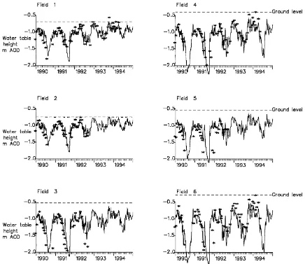
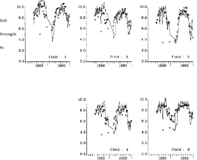
The DITCH model was applied to the conditions in the Broads area using the depth-dependent drainage Eq. (4). The meteorological data and the observed daily ditch levels for the relevant fields were used to model the water tables in the centre of each of the six monitored fields (Fig. 1). Visually, the results show excellent agreement between the model and the ob-servations. A statistical evaluation of the whole set of model results, which thus included the ability of the model to represent the variation both between fields and within fields, gave a correlation coefficient be-tween the modelled and observed water tables of 0.69, which was considered to be an excellent confirmation of the model. The model efficiency criterion (Loague and Green, 1991), for the same data set was 0.44, which again was considered to indicate an acceptable level of model performance.
4.2. Southlake
Fig. 1. Comparison of observed (*) and modelled (––––) water tables for the six monitored fields, in the Halvergate area of the Broads ESA, Eastern UK, 1990–1994. AOD indicates Above Ordnance Datum – mean sea level.
the dipwell data had suggested a continuity between the two layers in the profile. Direct measurement of the hydraulic conductivity of the peat subsoil, using the single auger hole technique indicated a subsoil conductivity of the order of 1–2 m/day.
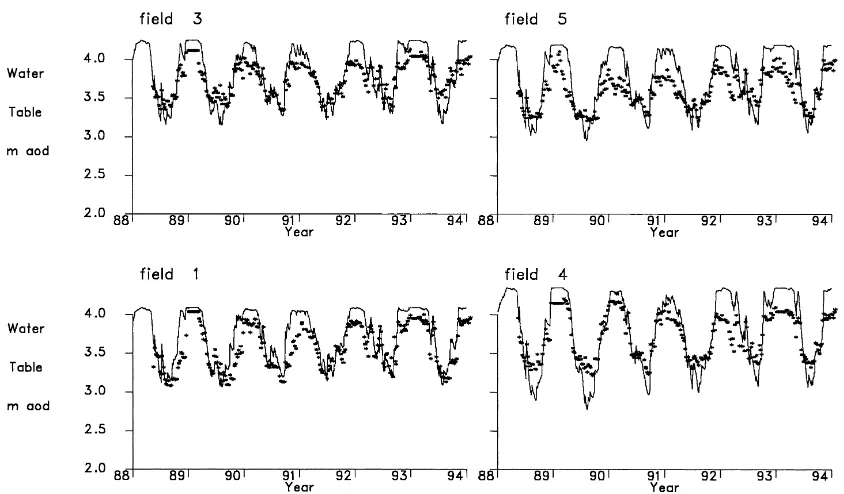
The observed gauge board heights at the outlet sluice were used to define the input boundary condi-tions. The modelled water tables were compared to the observed data (Fig. 2) for the recording period. Visual inspection of the model results showed that they were in general very close to observations. In particular, the model simulated the lowest depth to which the water table fell in the middle of the summer
in the last three years of the study. The same compar-ison was not possible for the first three years, during which the field data did not record deeper water ta-bles because of the shallow nature of the recording locations. The biggest divergence was that the model did not accurately reproduce the depths of flooding caused by the very high ditch levels.
Fig. 2. Comparison of observed (*) and modelled water tables, (solid line) for four of the monitored fields at Southlake Moor in the Somerset levels and Moors ESA, SW England, 1988–1994.
5. Estimation of soil surface strength
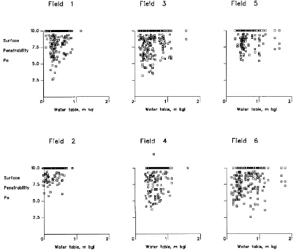
As the ability of birds to probe the soil for food is a major factor in the choice of sites for breeding, the estimation of soil surface strength is required to iden-tify site suitability for bird feeding needs (Tickner and Evans, 1991). For many soils, there is a relatively well defined relationship between soil strength and water content. As a first approximation, soil water content at the surface is also correlated with the water table depth from the surface, so a relationship between soil strength and water table offers the possibility of mod-elling the suitability of the soil for feeding by birds. This relationship cannot, however, be established from a priori principles, and must be calibrated from field observation.
The penetration resistance of the soil is a measure of the difficulty that a bird might be expected to have in feeding. For work specifically related to bird beak penetration, a special penetrometer has been devised (Green, 1986) which records the force required to push a narrow cylinder into the soil a distance of 100 mm, and so mimics the behaviour of a bird beak. At both
sites, the soil surface strength was recorded when-ever the auger holes were read using this penetrome-ter. On each occasion eight replicate measurements of soil strength were taken at three locations within each field.
Fig. 3. Relationships between soil strength and water table depth for each of the monitored fields in the Halvergate area of the Broads ESA.
The results also serve to emphasise the impact of and agricultural management practice affecting the value of land for ecological purposes.
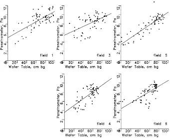
These results contrast with those obtained at South-lake Moor, (Fig. 4) where a clear correlation between water table depth and soil surface strength has been observed, for all the fields in the study area. The over-all correlation of 0.69 was considered to be remarkably good, especially when the other (often short term) fac-tors that can effect soil penetrability are considered. For Southlake it was, thus, possible to estimate soil surface strength from the water table position. Linear regression was used to estimate the relationship be-tween the two variables, and the estimated pattern of soil surface strength was shown to follow the observed
pattern (Fig. 5). These data show the pattern of be-haviour that is expected, being harder in the late sum-mer, coming to their softest in the winter, and gradu-ally hardening again during the summer, this pattern of behaviour being repeated for all the fields.
6. Estimation of surface flooding
Fig. 4. Relationships between soil strength and water table depth, for the five monitored fields at Southlake Moor in the Somerset levels and Moors ESA.
so estimate the soil water regime at all locations within the field, a simpler alternative is to assume that the water table is approximately flat, and that the area of the field that is flooded is defined by the intersection of this modelled water table height and the cumulative distribution of heights. Data presented by Armstrong and Rose (1998a) demonstrate the essentially flat na-ture of the water table. The DITCH model, thus, sim-ply takes the predicted water table height in the centre of the field, and then identifies the intersection of that height value with the cumulative frequency curve, to give an estimate of the extent of surface flooding in the field at any one time.
To implement this approach, it is essential to have some measure of the microtopographic roughness of the area modelled, ideally, as a cumulative frequency curve. Collection of these data requires measurement not only of the gross topographic features of the site, but also measurement of the microtopography. It was found that this information is best given by a series
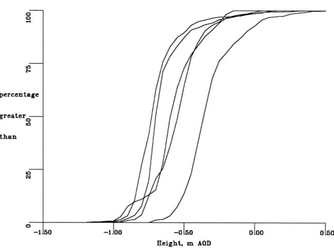
of closely measured transects, which give sample estimates for the whole field, rather than systematic surveys which tend to define only the macrotopo-graphic features. Fig. 6 shows the cumulative distribu-tions of surface heights for the six monitored fields in the Broads ESA. These are roughly Gaussian in their form, and so it is suggested that for more general ap-plication of the DITCH model, and in order to move away from the need to collect a large amount of to-pographic data, the cumulative frequency distribution could be replaced by its mean and standard.
Fig. 5. Observed (*) values of soil penetrability and those predicted by the DITCH model, for the monitored fields, in Southlake Moor in the Somerset Levels and Moors ESA, 1989–90.
7. Use of the model to evaluate management options
The DITCH model thus produces information about soil water regime, soil surface strength, and flooded area. The model was then used to evaluate a num-ber of alternative management options in these two areas.
7.1. Halvergate
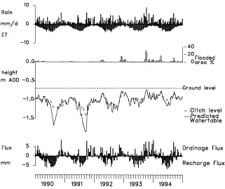
The model was used to examine the effectiveness of the various tiers of management on the water regimes of the Halvergate soils. In the implementation of the DITCH model the predicted water tables and surface flooding conditions were plotted on one graph (Fig. 7). In addition, to aid interpretation, the basic
hydro-logical variables of rainfall, evapotranspiration were plotted, and also the drainage fluxes which immedi-ately identified periods of recharge and drainage.
The model was run for a 16 year period, from 1979 to 1994, using the observed values for the hydraulic conductivity from the Halvergate area. and adopting three different ditch water level regimes representative of the three tiers of management relating to the ESA prescriptions:
• Tier 1. Ditch levels at 1.5 m below ground level from 1 January to 30 March, at 1.0 m below ground level 1 April to 30 October, and at 1.5 m below ground level 1 November to 31 December.
Fig. 6. Observed cumulative distributions of surface topographic heights for the six monitored fields in the Halvergate area of the Broads ESA.
at 45 cm below ground level until 30 October, and thereafter at 1.2 m below field level.
• Tier 3. Water levels are held at mean field level from 1 January to 30 April; at 45 cm below field level from 1 May to 30 October, then rising to mean field level by 1 December, and remaining at that level until the end of the year.
The mean in-field water tables simulated by the model over the 16 year run of rainfall data whilst subject to the 3 different levels of management are shown in Fig. 8, for each water management option. These results show the dramatic effect on in-field water regimes that are created by the different tiers of management. In particular, the adoption of high water levels in the Tier 3 levels results in the water table fluctuating only in the upper, conductive, layers of the soil, so that the field and ditch levels are closely tied together. By contrast, where the ditch levels fall in summer, the zone of water movement becomes concentrated in the lower impermeable layers, and the field and ditch wa-ter levels become effective disconnected, as the soil is then unable to transmit sufficient water to maintain
the water levels in the face of continuing evaporative demand.
7.2. Southlake
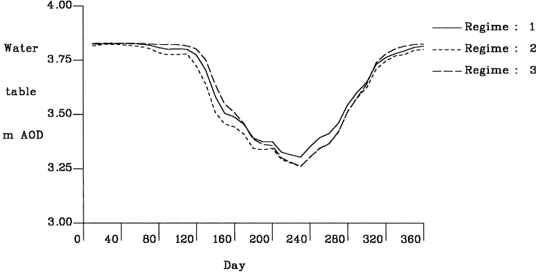
Lastly, the model was used to examine some of the effects of the water management prescriptions in the Somerset Levels and Moors ESA (Fig. 9). It was con-sidered that the model had fitted the data sufficiently well to be used to identify the impacts of these vari-ous regimes on the water levels within the field. The model was thus used to simulate the water table under both Tier 3 and under ‘normal conditions’, i.e., un-modified by the current ESA agreements, and under the current Tier 2 levels. The model was then run to represent a 10 year period, to produce a sequence of water tables for the three conditions. The mean results for all three water regimes are shown in Fig. 10, and as soil strengths in Fig. 11.
‘un-Fig. 7. Example application of the DITCH model to the Halvergate area of the Broads ESA, showing observed ditch levels (dashed line), predicted water tables (solid line) and surface flooding percentages (histograms). To aid interpretation, rainfall, evapotranspiration and drainage and recharge fluxes are also shown.
Fig. 8. Predicted mean water tables in response to the levels of ditch management (average of 20 modelled years) at the Halvergate site in the Broads ESA.
altered’ regime, with the effect being greatest in the spring and early summer. In the later part of the sum-mer the effects of evapotranspiration become domi-nant, reducing the effect the ditch levels have on the
Fig. 9. Example application of the DITCH model to the Southlake area: ditch levels (––––) and predicted water tables (solid line). To aid interpretation, rainfall, evapotranspiration and drainage fluxes are also shown.
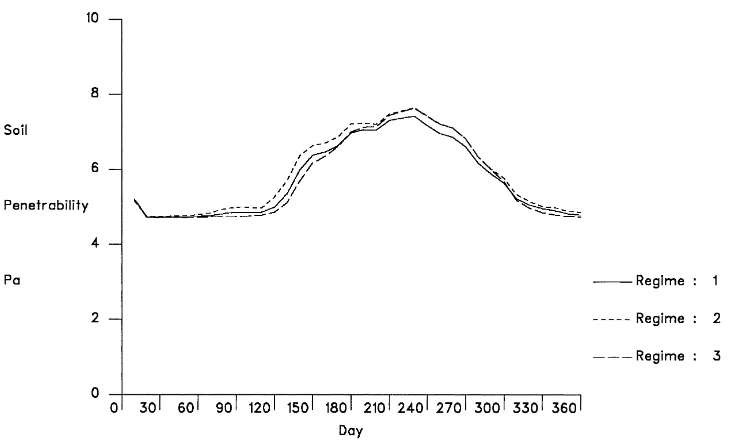
Fig. 11. Mean soil strength at Southlake Moor in the Somerset levels and Moors ESA, predicted for each of the three ditch management options.
regime is always the winter saturation and the sum-mer period of drying out. However, the effect in the centre of the field in terms of changing from the ‘old regime’ (Regime 2 in Figs. 10 and 11) to the new Tier 3 regimes with raised water levels in the ditches, is to delay the start of the spring drying out phase by an average of 20 days.
8. Conclusions
This paper has shown that a hydrological budget model can be used effectively to estimate the soil water and ditch regimes where those ditch levels are being manipulated. The validation tests of the models using the two data sets suggest that the model offers a good representation of the system.
However, the results also show that the effects of ditch management options are not easily converted into impacts in the centre of the fields. The small impacts identified in Figs. 10 and 11 indicate that although the ditch regimes may alter, the effects in the centre of the fields are very much more subtle. Although these effects may seem small, they are concentrated at the critical time of the year both for plants and for bird
life. Whether this effect is sufficient to achieve the re-quired ecological objectives is the subject of on-going research. If the effects are not sufficient, then hydro-logical manipulation of sites to achieve or maintain wetland status may require more active intervention on the within-field regimes.
Acknowledgements
References
Armstrong, A.C., 1983. The Measurement of watertable levels in structured clay soils by means of open auger holes. Earth Surface Processes 8, 183–187.
Armstrong, A.C., 1993. Modelling the response of in-field water tables to ditch levels imposed for ecological aims, a theoretical analysis. Agric. Ecosystems Environ. 43, 345–351.
Armstrong, A.C., Portwood, A.M., Castle, D.A., 1993. Simple models to predict field soil water regimes in the presence of ditch water levels managed for environmental aims. Transactions, Workshop on subsurface drainage simulation models. 15th International Congress on Irrigation and Drainage (ICID), The Hague, The Netherlands, 147–157.
Armstrong, A.C., Rose, S.C., 1998a. Managing water for wetland ecosystems: a case study. In: Joyce, C.B., Wade, P.M. (Eds.), European wet grasslands: management and restoration, Wiley, pp 201–214.
Armstrong, A.C., Rose, S.C., 1989b. Ditch water levels maintained for environmental aims: effects on field soil water regimes, MSS submitted to Hydrology and Earth System Sciences. Avery, B.W., 1955. The soils of the Glastonbury district of
Somerset, Memoirs of the Soil Survey of Great Britain, Sheet 296. HMSO, London, 131pp.
Belmans, C., Wesseling, J.G., Feddes, R.A., 1983. Simulation of the water balance of a cropped soil: SWATRE. J. Hydrol. 63, 271–286.
Clayden, B., Hollis, J.M., 1984. Criteria for differentiating soil series, Soil Survey Technical Monograph 17, Harpenden, Herts. Green, R.E., 1986. The management of lowland wet grassland for breeding waders. Unpublished Report, Royal Society for the Protection of Birds, Sandy, Beds, UK.
Green, R.E., 1988. Effects of environmental factors on the timing and success of breeding of common snipe Gallinago Gallinago (Aves: Scolopacidae). J. Appl. Ecol. 25, 79–93.
Loague, K., Green, R.E., 1991. Statistical and graphical methods for evaluating solute transport models: overview and application. J. Contaminant Hydrol. 7, 51–73.
MAFF, 1989. Environmentally Sensitive Areas (first report). HMSO London, 50pp.
MAFF, 1991a. The Broads Environmentally Sensitive Area, report of monitoring 1991. HMSO, London, 51pp.
MAFF, 1991b. The Somerset Levels and Moors Environmentally Sensitive Area Report of Monitoring 1991. HMSO, London. Maltby, E., 1986. Waterlogged Wealth. Earthscan Publications,
London, 193pp.
Ritzema, H.P. (Ed.), 1994. Drainage Principles and applications. ILRI Publication 16 (2nd edn.). International Institute for Land Reclamation and Improvement, Wageningen, The Netherlands, 1125pp.
Skaggs, R.W., 1982. Field evaluation of a water management simulation model. Transactions. Am. Soc. Agric. Eng. 25, 666– 674.
Smedema, L.K., Rycroft, D.W., 1983. Land drainage: planning and design of agricultural drainage systems, Batsford Academic and Educational, London, 376pp.
Talman, A.J., 1980. Simple flow meters and watertable meters for field experiments. MAFF Land Drainage Service Technical Report 79/1. MAFF Publication, Pinner, 18pp.
Talman, A.J., 1983. A device for recording fluctuating water levels. J. Agric. Eng. Res. 28 273, 277.
Tickner, M.B., Evans, C.E., 1991. The management of lowland wet grasslands on RSPB reserves. Royal Society for the Protection of Birds, Sandy, Beds, UK 124pp.
Van Schilfgaarde, J., 1974. Drainage for Agriculture. American Society of Agronomy, Madison, Wisconsin, 700pp.
Wesseling, J., 1973. Flow into drains. Chapter 8 of Drainage Principles and Applications, International Institute for Land Reclamation and Improvement, Publication 16, vol. II, p. 1– 56.
Youngs, E.G., 1965. Horizontal seepage through unconfined aquifers with hydraulic conductivity varying with depth. J. Hydrol. 3, 283–296.