Estimation of mean monthly solar global radiation as
a function of temperature
Francisco Meza
a,∗, Eduardo Varas
b,1aDepartamento de Ciencias de Recursos Naturales, Pontificia Universidad Católica de Chile, Casilla 306, Correo 22, Santiago, Chile bDepartamento de Ingenier´ıa Hidráulica y Ambiental, Pontificia Universidad Católica de Chile, Casilla 306, Correo 22, Santiago, Chile
Received 14 December 1998; received in revised form 11 August 1999; accepted 13 August 1999
Abstract
Solar radiation is the primary energy source for all physical and biochemical processes that take place on earth. Energy balances are a key feature of processes such as temperature changes, snow melt, carbon fixation through photosynthesis in plants, evaporation, wind intensity and other biophysical processes. Solar radiation level is sometimes recorded, but generally it needs to be estimated by empirical models based on frequently available meteorological records such as hours of sunshine or temperature.
This paper evaluates the behavior of two empirical models based on the difference between maximum and minimum temperatures and compares results with a model based on sunshine hours. This work concludes that empirical models based on temperature have a larger coefficient of determination than the model based on cloud cover for the normal conditions of Chile. These models are easy to use in any location if the parameters are correctly adjusted. In addition, probability distribution functions and confidence intervals for solar radiation estimates using stochastic modeling of temperature differences were calculated. ©2000 Published by Elsevier Science B.V. All rights reserved.
Keywords:Solar radiation; Temperature; Random variable; Fourier series
1. Introduction
In some cases a record of global solar radiation (RG) using instruments such as pyranometers or actinome-ters is available, however, there are many meteorolog-ical stations which do not measure solar radiation, but do register other variables such as precipitation, pres-sure and temperature. For this reason, this paper
eval-∗Corresponding author. Fax:+56-2-553-92-31.
E-mail addresses:[email protected] (F. Meza), [email protected] (E. Varas).
1Fax+56-2-686-58-76.
uates proposed mathematical models to estimate so-lar radiation as a function of temperature differences and compares their performance with models based on sunshine hours.
Solar radiation is the principal energy source for physical, biological and chemical processes, such as, snow melt, plant photosynthesis, evaporation, crop growth and is also a variable needed for biophysical models to evaluate risk of forest fires, hydrological simulation models and mathematical models of natu-ral processes. Hence, in many occasions, a record of observed solar radiation or an estimate of radiation is required.
2. Model description
Extra-terrestrial solar radiation, also known as An-got radiation (RA, MJ m−2day−1) can be calculated as a function of the distance from the sun to earth (d, km), the mean distance sun–earth (dm, km), latitude
(φ, rad), solar declination (δ, rad) and solar angle at sunrise (sunset) (Hs, rad) using the following
expres-sion (Romo and Arteaga, 1983):
RA=
Using the preceding relationship, solar radiation can be calculated for any point in the earth’s outer atmo-sphere for each day of the year as a function of latitude and solar declination. However, gases and clouds in-troduce changes to both magnitude and spectral com-position of solar radiation.
2.1. Angström model, 1924
Since the beginning of the century, efforts have been made to estimate solar radiation as a function of extra-terrestrial solar radiation and the state of the atmosphere (Castillo and Santibáñez, 1981). The pa-rameter most commonly used is hours of sunshine. Usually, the ratio of global solar radiation to Angot ra-diation is correlated to the ratio of effective sunshine hours to total possible sunshine hours.
Effective sunshine hours (n) are measured with a heliograph (Mart´ınez-Lozano et al., 1984). Although this instrument has a threshold, under which sunshine is not recorded, this error is not significant when esti-mating daily solar radiation.
Angström (1924), suggested a simple linear re-lationship to estimate global solar radiation (RG, MJ m−2day−1) as a function of Angot radiation, actual sunshine hours (n) and potential or theoretical sunshine hours (N).
RG RA
=a+bn
N (2)
Angström suggested values of 0.2 and 0.5 for empirical coefficients a and b respectively. Other authors, such as Bennett (1962), Davies (1965),
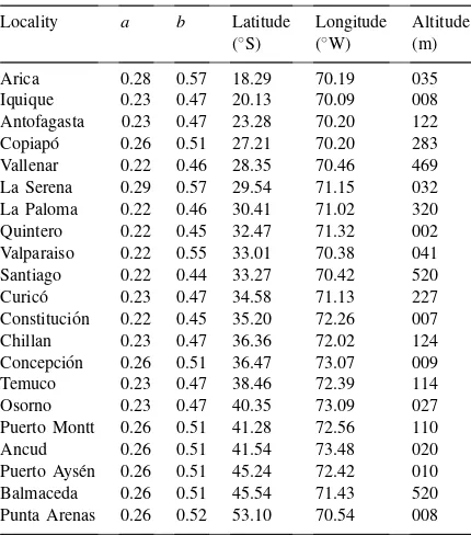
Table 1
Angström coefficients (aandb) recommended for Chilean locali-ties. (Castillo and Santib´añez, 1981)
Locality a b Latitude Longitude Altitude (◦S) (◦W) (m)
Arica 0.28 0.57 18.29 70.19 035
Iquique 0.23 0.47 20.13 70.09 008 Antofagasta 0.23 0.47 23.28 70.20 122 Copiap´o 0.26 0.51 27.21 70.20 283 Vallenar 0.22 0.46 28.35 70.46 469 La Serena 0.29 0.57 29.54 71.15 032 La Paloma 0.22 0.46 30.41 71.02 320 Quintero 0.22 0.45 32.47 71.32 002 Valparaiso 0.22 0.55 33.01 70.38 041 Santiago 0.22 0.44 33.27 70.42 520 Curic´o 0.23 0.47 34.58 71.13 227 Constituci´on 0.22 0.45 35.20 72.26 007 Chillan 0.23 0.47 36.36 72.02 124 Concepci´on 0.26 0.51 36.47 73.07 009 Temuco 0.23 0.47 38.46 72.39 114 Osorno 0.23 0.47 40.35 73.09 027 Puerto Montt 0.26 0.51 41.28 72.56 110
Ancud 0.26 0.51 41.54 73.48 020
Puerto Ays´en 0.26 0.51 45.24 72.42 010 Balmaceda 0.26 0.51 45.54 71.43 520 Punta Arenas 0.26 0.52 53.10 70.54 008
Monteith (1966), Penman (1948), and Turc (1961) have calibrated this expression for different places. Coefficients can vary significantly as Doorenbos and Pruitt (1975) show. In Chile, Castillo and San-tibáñez (1981), have recommended the values given in Table 1.
2.2. Bristow–Campbell model, 1984
Furthermore, if the heat flow towards the soil is neglected, one can find the ratio of sensible heat to latent heat or Bowen ratio, on a daily basis (Campbell, 1977). Sensible heat is responsible for temperature variations, so it is possible to obtain a relationship between temperature differences and solar radiation, being temperature a reflection of radiation balance.
Using this argument, Bristow and Campbell (1984), suggested the following relationship for dailyRG, as a function of daily RA and the difference between maximum and minimum temperatures (1T,◦C):
RG RA
=Ah1−exp(−B1TC)i (3)
Athough coefficients A,B andC are empirical, they have some physical meaning. CoefficientArepresents the maximum radiation that can be expected on a clear day. CoefficientsBandCcontrol the rate at whichA
is approached as the temperature difference increases. Values most frequently reported for these coefficients are 0.7 forA, the range 0.004 to 0.010 forBand 2.4 forC.
Since clear days present large temperature differ-encesAtends to be the ratio between global solar radi-ation and Angot radiradi-ation, hence the sum of Angström coefficientsaandbtends to be similar toA.
2.3. Allen model, 1997
Allen (1997), suggested the use of a self-calibrating model to estimate mean monthly global solar radiation following the work of Hargreaves and Samani (1982). He suggested that the mean dailyRGcan be estimated
as a function ofRA, mean monthly maximum(TM,◦C)
and minimum temperatures (Tm,◦C). RG
RA
=Kr(TM−Tm)0.5 (4)
Previously, Allen (1995), had expressed the empiri-cal coefficient (Kr) as a function of the ratio of atmo-spheric pressure at the site (P, kPa) and at sea level (P0, 101.3 kPa) as follows:
In his work, Allen suggested values of 0.17 for interior regions and 0.20 for coastal regions for the empirical coefficientKra.
3. Climatic data
In order to compare the behavior of the different models, monthly climatological data of 21 stations representing different climatic regions of Chile were collected. Data ranged from Arica (latitude 18.3◦S) to Punta Arenas (53.1◦S) and was registered between the years 1971 and 1992.
Selected meteorological variables wereTM,Tm,P,
mean monthly degree of cloud cover (x) andRG.
For the locations mentioned in Table 1, monthly val-ues of maximum and minimum temperatures, cloud cover and atmospheric pressure for each year in the period 1971 to 1992, were available. Unfortunately, for global solar radiation only the average value for each month in that period was available and monthly radiation values for each year were impossible to ob-tain from Dirección Meteorológica de Chile.
In addition to the above, data from La Paloma sta-tion was collected to compare the behaviour of models based on temperature differences when they are ap-plied to estimate monthly global solar radiation. The selected meteorological variables in this case wereTM,
Tm,P, andRGbetween the years 1971 and 1978.
Finally, data from Santiago station was used to compare the behaviour of Bristow–Campbell and Allen models when they are applied to estimate daily global solar radiation. The meteorological variables were dailyTM,Tm,P, andRG.
4. Models applied to mean monthly data
The extension of the reviewed models to apply them to monthly averages requires some explanation. The Angström model was originally derived for daily so-lar radiation and hours of sunshine. Nonetheless, be-ing a linear function it can be readily applied to mean monthly data since the expected value of a sum is equal to the summation of the expected values. Allen’s model was derived for monthly data so it can readily be used. However, the Bristow–Campbell model is de-fined for daily data and has no evident extrapolation to mean monthly values. For this reason, one can ex-pect to find a new set of coefficients when the same expression is applied to monthly data.
radiation was calculated at each site, using the ex-pressions and empirical coefficients suggested by Angström (1924), Bristow and Campbell (1984), and Allen (1995). Results show that models using the coefficients proposed in the literature do not esti-mate correctly the historical average in each location. The slope of the relationship between calculated and observed radiation is significantly different from unity. This is especially notorious in the case of the Bristow–Campbell model, although this result was ex-pected since the coefficients suggested by the authors are applicable to daily data.
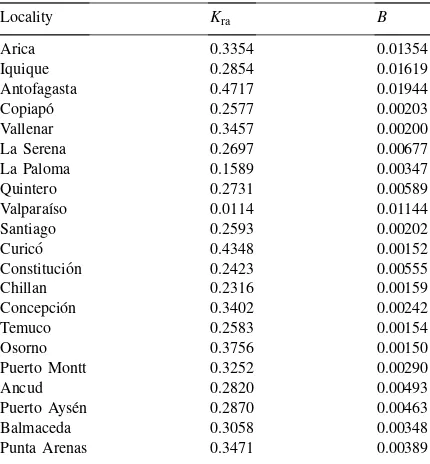
Given the results, it was necessary to change the Allen and Bristow–Campbell model coefficients to obtain a better fit, following the idea suggested by Castillo and Santibáñez (1981) for the Angström model. Least squares coefficients, which minimize the sum of square errors for each location were calculated and included in Table 2.
Due to the fact that monthly solar radiation values, were not available for each year, as mentioned in the section about climatic data, theA andCcoefficients of Bristow–Campbell model were assumed fixed and theBcoefficient was adjusted to minimize the square
Table 2
Adjusted coefficients (KraandB) of Allen and Bristow–Campbell models
La Serena 0.2697 0.00677
La Paloma 0.1589 0.00347
Quintero 0.2731 0.00589
Puerto Montt 0.3252 0.00290
Ancud 0.2820 0.00493
Puerto Ays´en 0.2870 0.00463
Balmaceda 0.3058 0.00348
Punta Arenas 0.3471 0.00389
Table 3
Regression between calculated and observed mean monthly global solar radiation using adjusted parameters of 20 Chilean localities
Model Slope Upper Lower R2
limit. (95%) limit. (95%)
Angström 0.959 0.970 0.939 0.892
Allen 0.999 1.010 0.990 0.961
Bristow–Campbell 1.152 1.170 1.138 0.928
errors. The available data made it impossible to study the contribution of coefficientsAandC. However,A
represents the maximum radiation on a clear day and its value represents the observed data reasonably well. Moreover, a change in coefficientC does not affect significantly the calculated global solar radiation.
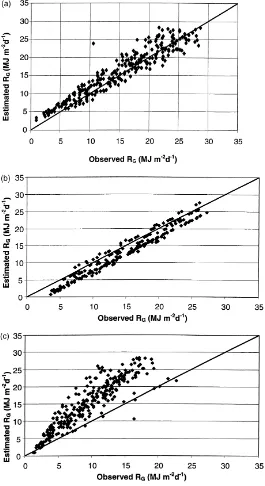
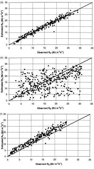
Observed and calculated values for different locations and models are shown in Fig. 1. In this figure the improvement in the relationships when us-ing locally calibrated coefficients can be appreciated. The Angström model results using the coefficients proposed by Castillo and Santibáñez (1981) are also included for comparison. Slopes of the different mod-els and the coefficients of determination are given in Table 3.
Allen’s model presents the best relationship. It has a higher coefficient of determination and the slope is equal to unity with 90% confidence interval. The Bristow–Campbell model tends to under-estimate global solar radiation but explains a large proportion of sample variance. The Angström model fit the data poorer than the other two.
4.1. Models applied to monthly data.
Since the available data of global solar radiation for most stations is only the average value for each month, it was necessary to examine if the relationships with the adjusted coefficients represent accurately the monthly values for each year. One station available with monthly global solar radiation data, is La Paloma. In this case the models with the adjusted coefficients derived with the average monthly values were used to estimate monthly global solar radiation for each year. A comparison between estimated monthly values for La Paloma, compared to observed monthly values is shown in Table 4.
Table 4
Regression between calculated and observed monthly global solar radiation at La Paloma station
Model Slope Upper Lower R2
limit. (95%) limit. (95%)
Allen 1.000 1.010 0.990 0.97
Bristow–Campbell 0.994 1.006 0.982 0.96
models. Allen’s model presents the best relationship between observed and calculated monthly solar global radiation because it explains a large proportion of the sample variance. In both models the slope is equal to unity with 90 % confidence interval. This verifies that the models can be used to estimate monthly values for different years.
4.2. Global solar radiation distribution functions
A probability distribution function for global solar radiation was obtained as a derived distribution, when radiation is expressed as a function of temperature dif-ferences and temperature difdif-ferences are expressed as a Fourier series with a random component. This ran-dom error was found to be a ranran-dom variable with nor-mal distribution. This hypothesis was tested in both for the Bristow–Campbell and the Allen models using the Anderson–Darling test for normal distribution. Once a distribution model for solar radiation is calculated, confidence intervals for estimates can be computed.
4.3. Temperature difference modelling.
Temperature has a marked seasonal variation due to periodicity in the earth’s orbit about the sun. For this reason temperature variations can be represented us-ing mathematical cyclic functions. In this paper, dif-ferences between maximum and minimum tempera-tures were modelled using a Fourier series once the stationary component was removed, as suggested by Van Wijk and De Vries (1966) and Campbell and Nor-man (1997). These authors applied Fourier series with one term to represent air temperatures.
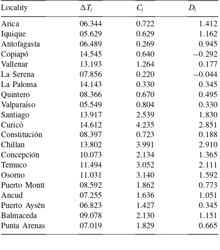
The1Tin locationiand monthj(1Tij,◦C) can be
expressed as a function of mean annual1Tin location
i(1Ti,◦C), Fourier series coefficients at locationi(Ci, Di) and an error or residual in locationiand monthj
(Eij,◦C) as follows:
Table 5
Average temperatures (1Ti) and Fourier series coefficientsCiand
Di of 20 Chilean localities
Locality 1Ti Ci Di
Arica 06.344 0.722 1.412
Iquique 05.629 0.629 1.162
Antofagasta 06.489 0.269 0.945
Copiap´o 14.545 0.640 −0.292
Vallenar 13.193 1.264 0.177
La Serena 07.856 0.220 −0.044
La Paloma 14.143 0.330 0.345
Quintero 08.366 0.670 0.495
Valpara´ıso 05.549 0.804 0.330
Santiago 13.917 2.539 1.830
Curic´o 14.612 4.235 2.851
Constituci´on 08.397 0.723 0.188
Chillan 13.802 3.991 2.910
Concepci´on 10.073 2.134 1.365
Temuco 11.494 3.052 2.111
Osorno 11.031 3.140 1.592
Puerto Montt 08.592 1.862 0.773
Ancud 07.255 1.636 1.051
Puerto Ays´en 06.823 1.427 0.345
Balmaceda 09.078 2.130 1.151
Punta Arenas 07.019 1.829 0.665
1Tij=1Ti +Cicos
The coefficientsCiandDi are given in Table 5 for the
sites used in this work.
4.4. Probability distribution functions
IfXis a continuous random variable with a proba-bility density functionf(x) andYis a monotonic func-tion ofX, then the probability function of Y can be obtained multiplying the inverse function by the abso-lute value of the Jacobian of the transformation (J) or determinant of the first derivative ofw(y) with respect toX(Walpole and Myers, 1992):
g(y)=f[w(y)]|J| (7)
Using this procedure probability density and proba-bility distribution functions forRGestimated by Allen
4.5. Bristow–Campbell model
In this case the distribution function is calculated using Eq. (3) and replacing1Tij for its expression in
terms of annual 1T in each location and the corre-sponding Fourier series coefficients. Combining both the expressions, an equation for the residuals is ob-tained. Residuals were found to be well represented by a normal distribution model, so the probability dis-tribution of the errors was assumed known. The distri-bution hypothesis was tested using Anderson–Darling test.
The probability density function for solar radiation following Eq. (7), is equal to the product of the normal density function evaluated at the residuals for location
iand monthj and the absolute value of the transfor-mation Jacobian (Eq. (8)). The residuals are given in this case by Eq. (9) and the first derivative by Eq. (10).
g(RGij)=[J]f(RGij) (8)
The residuals are given by the following equation ex-pressed as a function of terms already defined:
Eij=
The first derivative is:
|J| =
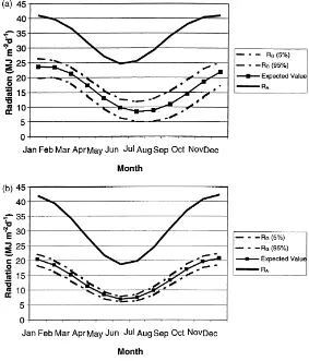
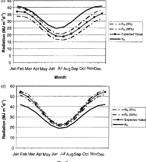
The cumulative distribution function (CDF) is ob-tained by integrating the probability density function. The CDF was evaluated numerically, using very small intervals and the trapezoidal integration method, to define confidence intervals for global solar radia-tion. Results for two locations Arica and Vallenar are shown graphically in Fig. 2 (a,b).
4.6. Allen’s model
Similarly, for Allen’s model, 1997, the probability density function is obtained using Eq. (4) and replac-ing1Tij for its expression in terms of annual1Tin
each location and the corresponding Fourier series co-efficients (Eq. (6)). Residuals in this case were also found to be well represented by a normal distribution model, so the probability distribution of errors was assumed known.
The probability density function for solar radiation is shown in Eq. (8).The residuals are given in this case by Eq. (11) and the first derivative by Eq. (12):
Eij=
The CDF is obtained integrating the probability den-sity function. It was evaluated numerically to define confidence intervals for global solar radiation. Re-sults for Arica and Vallenar are shown graphically in Fig. 2(c,d). The expected value for global solar radiation given by the CDF using Allen’s model are higher than the Angot radiation because the limits of integration derived in this case were zero and infinite. On the other hand, the CDF using Bristow-Campbell model have clear and defined limits which are zero and A times the Angot radiation. For this reason the CDF obtained with Bristow–Campbell model is more accurate and has smaller confidence intervals.
5. Models applied to daily data
5.1. Allen’s model
Fig. 2. (a) Expected values and confidence limits (5 and 95%) of daily mean global radiation using Bristow-Campbell model and Angot radiation for Arica; (b) Expected value and confidence limits (5 and 95 %) of daily mean global radiation using Bristow-Campbell model and Angot radiation for Vallenar; (c) Expected value and confidence limits (5 and 95 %) of daily mean global radiation using Allen model and Angot radiation for Arica; (d) Expected value and confidence limits (5 and 95%) of daily mean global radiation using Allen model and Angot radiation for Vallenar.
This model tends to over estimate global solar ra-diation in a daily basis, and frequently estimates radi-ation in excess of the extra-terrestrial radiradi-ation, since the condition expressed by Eq. (13) is fulfilled. This model does not have a limit for the estimated solar radiation.
1T > P0 (Kra)2P
(13)
This condition is frequently true when the model is applied to points located in interior regions which usually experience large daily temperature variations.
Even though Allen’s model has a larger coeffi-cient of determination, the slope is clearly less than unity, indicating that the model over-estimates solar radiation.
5.2. Bristow–Campbell model
This model is defined solely in terms of temperature differences and is thus simpler to apply. The value for
Fig. 2 (Continued).
Table 6
Regression between calculated and observed daily global solar radiation at Santiago station
Model Slope Upper Lower R2
limit. (95%) limit. (95%)
Allen 0.561 0.549 0.571 0.85
Bristow–Campbell 1.090 0.979 1.202 0.79
The behavior of the Bristow–Campbell model is more consistent and reliable, since it has an upper limit given by parameter A. The regression analysis shows that the Bristow–Campbell model performs better (Table 6). On the other hand, Bristow–Campbell model gives consistently a better estimate when applied to daily data.
6. Conclusions
Empirical models to estimate global solar radia-tion are a convenient tool if the parameters can be calibrated for different locations. These models have the advantage of using meteorological data which are commonly available.
of general application. Temperature variation can be modelled by Fourier series and confidence intervals for global solar radiation estimates can be obtained using derived distribution procedures. Both the models have limitations when applied to daily data. Solar radiation at locations with large temperature differences are not correctly modelled using Allen procedure and the Bristow–Campbell model had a better performance.
References
Allen, R., 1995. Evaluation of procedures of estimating mean monthly solar radiation from air temperature. FAO, Rome. Allen, R., 1997. Self-calibrating method for estimating solar
radiation from air temperature. J. Hydrol. Eng. 2, 56–67. Angström, A., 1924. Solar and terrestrial radiation. Q.J.R.
Meteorol. Soc. 50, 121–125.
Bennett, I., 1962. A method of preparing maps of mean daily global radiation. Arch. Meteorol. Geophys. Bioklimatol Ser. B 13, 216–248.
Bristow, K., Campbell, G., 1984. On the relationship between incoming solar radiation and daily maximum and minimum temperature. Agric. For. Meteorol. 31, 159–166.
Castillo, H., Santibáñez, F., 1981. Evaluación de la radiación solar global y luminosidad en Chile I. Calibración de fórmulas para
estimar radiación solar global diaria. Agricultura Técnica 41, 145–152.
Campbell, G., 1977. An Introduction to Environmental Biophysics. Springer, New York.
Campbell, G., Norman, J., 1997. An Introduction to Environmental Biophysics. Soils/AOS 532. Pullman WA.
Chang, J.-H., 1968. Climate and Agriculture. Aldine Publishing. Chicago.
Davies, J.A., 1965. Estimation of insolation for West Africa. Q.J.R. Meteorol. Soc. 91, 359–363.
Doorenbos, J., Pruitt, W., 1975. Crop water requierements, Irrigation and drainage paper, 24. FAO, Rome.
Hargreaves, G., Samani, Z., 1982. Estimating potential evapotranspiration. J. Irrig. Drain. Eng. ASCE. 108, 225–230. Mart´ınez-Lozano, J., Tena, F., Onrubia, J., De la Rubia, J., 1984. The historical evolution of Angström formula and its modifications: review and bibliography. Agric. For. Meteorol. 33, 109–128.
Monteith, J.L., 1966. Local differences in the attenuation of solar radiation over Britain. Q.J.R. Meteorol. Soc. 92, 254–262. Penman, H.L., 1948. Natural evaporation from open water, bare
soil and grass. Proc. R. Soc. London Ser. A. 193, 120–145. Romo, J., Arteaga, R., 1983. Meteorolog´ıa Aplicada. Universidad
Autónoma de Chapingo. 442 pp.
Turc, L., 1961. Evaluation des besoins en eau d’irrigation. Evapotranspiration potentielle. Ann. Agron. 12, 13–49. Van Wijk, W., De Vries, D., (1966). Physics of Plant Environment,