Estimation of leaf area and its vertical distribution during growth period
J. Ross
a,∗, V. Ross
a, A. Koppel
b aTartu Observatory, 61602 Tõravere, Estonia bEstonian Agricultural University, 51014 Tartu, EstoniaReceived 19 July 1999; received in revised form 15 December 1999; accepted 17 December 1999
Abstract
A statistical interpolation method is proposed which allows calculation of the leaf area index LAI(t), the downward cumulative leaf area index L(z, t) and the canopy leaf area density u(z, t) as the functions of height and time for any day of the growth period. The method is based on three functions: probability density of stem height, interrelationship between stem height and stem foliage area, and the shape function of stem foliage vertical distribution. The method was elaborated in detail using phytometrical measurements carried out on willow coppice (Salix viminalis L.) during the growth period of 1998 in Tõravere, Estonia. The estimated values of u(z, t) and those calculated by the method differ by about 10–15%.
The interpolation model can be used when phytometrical data are available for certain days throughout the growing season. It could be applied to pure stands: young forests, orchard plantations, and maize, sorghum and cotton crops, etc. ©2000 Elsevier Science B.V. All rights reserved.
Keywords: Statistical interpolation method; Leaf area index; Vertical distribution of leaf area; Willow coppice
1. Introduction
The spatial distribution of canopy elements is an important factor in canopy–atmosphere exchange pro-cesses, and the knowledge of the vertical profile of leaf area serves as a critical input in the models of these processes. Using the simulation model ‘MAESTRO’, Wang and Jarvis (1990b) demonstrated that tree crown structure influences strongly canopy PAR absorption, photosynthesis and transpiration. The vertical distri-bution of canopy leaf area is characterized by the leaf area density (LAD) function u(z) (m2/m3) which is re-lated to another parameter of canopy foliage area — the downward cumulative leaf area index L(z).
∗Corresponding author. Tel.:+372-7-410-278;
fax:+372-7-410-205.
E-mail address: [email protected] (J. Ross).
The latter characteristic determines leaf area in m2/m2 ground area which is located in the upper canopy layer higher than the level z. The leaf area index LAI is single-sided leaf area in m2/m2 ground area of the whole canopy. The total leaf area of the individual stem in m2 is SP. The vertical distribution
of the foliage area of the individual stem is expressed by the function S(z) which determines foliage area in m2/m crown thickness at the height z.
A great number of papers have been published in which the vertical profiles of LAD of many species and canopies have been expressed showing that u(z) and S(z) are highly variable and dynamic functions. To compare LAD of individual plants with different heights or of different species at different times during the growth period, Ross and Ross (1969, 1996a), and Ross (1981) introduced the so-called shape function of the vertical distribution of the stem foliage, S*(z*). This function is determined in the interval of the
Table 1
Different models used for leaf area vertical distribution
Authors Species Modeled characteristic Model
Kinerson and Fritschen, 1971 Douglas fir S*(z) Triangle
Allen, 1974 Sorghum u(z) Parabolic
Chen et al., 1994 Poplar S(z) Sine and cosine
Stephens, 1969 Red pine S(z) Normal distribution
Borghetti et al., 1986 Douglas fir S(z) Normal distribution
Beadle et al., 1982 Scots pine S(z) Modified normal distribution
Massmann, 1982 Douglas fir S*(z*) Beta distribution
Wang and Jarvis, 1990a Sitka spruce S*(z*) Beta distribution
Wang et al., 1990 Radiata pine S*(z*) Beta distribution
Stenberg et al., 1993 Scots pine S*(z*) Beta distribution
Yang et al., 1993 Mixed pine L(z) Cumulative Weibull distribution
Gillespie et al., 1994 Young loblolly pine L(z) Cumulative Weibull distribution
relative height z* betweenz∗L and 1, where the rela-tive lower level of the canopy foliage z∗L during the growth period increases monotonically.
The function S*(z*) expresses the shape of S(z) in relative units and allows comparision of plants with a different height and at different points of time. Dif-ferent shapes of S*(z*) of many species are given by Ross (1981).
Several attempts have been made to fit S(z), S*(z*) or u(z) by some commonly used distribution functions (Table 1).
To simulate the asymmetric crown shape and LAD distribution inside the crown, Cescatti (1997a) elab-orated the flexible model FOREST and used it for modelling radiative transfer in discontinuous Norway spruce stand (Cescatti, 1997b).
The empirical parameters of different distribution functions are not constant, they change during the fo-liated period and also from year to year during forest growth.
Long-term productivity, photosynthesis etc. models require the knowledge of the input functions of L(z) or u(z) for the whole growth season. For their estima-tion, direct phytometrical measurement or indirect de-termination methods are needed. Such measurements are very tedious and time-consuming and can be car-ried out in field conditions with 2–3-weekly intervals at best. However, the time step of comprehensive bio-physical exchange and productivity models is usually much shorter, 1 h or day.
Hence the vertical distribution of LAD, u(z, t), and the downward cumulative leaf area index, L(z, t) as the functions of height z and time t should be considered,
and methods for estimation of u(z, t) or L(z, t) for different canopy types should be elaborated.
The aim of this paper is to develop a statistical interpolation method which allows determination of u(z, t), L(z, t) and LAI(t) for any time throughout the whole growth period. This method is based on
phytometrical measurements on sampling days tm
with 2–3-weekly intervals, on estimation of u(z, tm),
L(z, tm) and LAI(tm) for the days tm and on the
cal-culation of u(z, t), L(z, t) and LAI(t) for any day t of the growth period. The method is applicable for pure stands (young forests, orchard plantations, and maize, sorghum, cotton crops, etc.) and it has been tested on the willow coppice.
2. Interpolation method
The method includes the following steps.
(a) Estimation of the stem height probability density function fzP(zP) and fitting it by some known
distribu-tion. In many cases, the normal distribution, which is described by two parameters — meanhzPi and stan-dard deviation (STD)σszP— is applicable. For some
species (e.g. willow coppice) the height distribution function in a certain growth period can be bimodal and fzP should be fitted as the superposition of two
dis-tribution functions. During the growth period, mean and STD change, can be regarded as the functions of time. UsuallyhzP(t )iandσzP(t) are smooth functions
(b) Estimation of parameters for the correlation
function between the stem leaf area SP and stem
height zP. For willow coppice the following power
function can be used
SP(zP)=b0zPb, (1)
where b0 and b are empirical coefficients
describ-ing quite well correlation between leaf area and stem height. During the growth period, coefficients b0and
b change and can be fitted by polynomials as the func-tions of time, i.e.
where b0i and bi are polynomial coefficients.
Eqs. (1)–(3) allow calculation of the leaf area SP(zP, t) of the stem with the height zPat any time t of
the growth period, using data measured on sampling days.
(c) The most tedious step is estimation of the shape function of the stem leaf area vertical distribution
S∗ z∗ = zP
SP
S(z), (4)
where zPis stem height and z∗=z/zPis relative height.
The normalizing condition for S*(z*) is
Z 1
foliage at the bottom level. At the top of the plant, S(zP)=0 and S*(1)=0.
On selected days tm, sample stems with a
differ-ent height (taking into account the height distribution function fzP) are harvested. The stem is divided into
10 layers with the equal relative thickness1z*=0.1. The leaf area SL(z∗i, tm) in each layer is measured and
the relative leaf area S*(z∗i, tm) is calculated in
accor-dance with Eq. (4). Using the data set S*(z∗i, tm) of
all sample stems, the shape function S*(z*, tm) will be
estimated fitting the S*(z∗i, tm) by the polynomial
S∗(z∗, tm)= l X
i=0
ai(tm) z∗i, (6)
where aiare the polynomial coefficients which change
during the growth period.It should be noted that the fitting polynomial is valid in the intervalz∗L,1of the relative height z*.
To estimate the time dependence of S* we used the following procedure.
On sampling days tm, using the Eq. (4), we
calculate for the relative heightsz∗n=0.9, 0.8,. . ., zL
the values of S*(z∗n, tm) and use them for constructing
the function S*(z*, t). To determine the dependence of S* on time at the fixed relative height z∗
n we
employ approximation by the third order polynomial
S∗ zn∗, t=
Polynomial coefficients ak(zn∗) are regarded as the
functions of the relative height z* and will be approx-imated by the fifth order polynomial
ak z∗n
Finally, from Eqs. (6), (6a) and (7) we obtain
S∗ z∗, t=
The last equation allows calculation of the shape func-tion of the stem leaf area at any time of the growth period.
(d) The final step of the method is calculation of the canopy u(z, t), L(z, t) and LAI(t). Consider the canopy elemental layer with the thickness1z at the height z. Total leaf area in this layer consists of leaves from individual stems whose height zP>z. One stem with
the height zP>z contributes to the layer1z whose leaf
area, in accordance with Eq. (4), is
SP zp
zP
S∗ z∗.
At the height z the number of stems with the height zP
is NP(t) fzP (zP, t). The contribution of all stems with
To obtain total leaf area in the layer 1z one must summarize all stems with a different height. Finally, the canopy leaf area density u(z, t) at the height z and time t is
where zUis the upper level of the canopy foliage and
SP (zP, t) is given by Eqs. (1)–(3), and S*(z*, t), by
Eq. (6b).
The downward cumulative leaf area index L(z, t) and the leaf area index LAI(t) can be calculated by summarizing u(z, t) over z.
In conclusion, when one has a set of required phyto-metrical data for sampling days tmwithin the growth
period, interpolation method allows calculation of the canopy leaf area characteristics u(z, t), L(z, t) and LAI(t) for any day of the growth period.
3. Study area and methods
Phytometrical measurements were carried out dur-ing the vegetation period of 1998 in a willow coppice of Salix viminalis (L.), clone 78021, located close to Tartu Observatory, Tõravere (58◦16′N, 26◦28′E, 70 m asl), Estonia. For more details see (Koppel et al., 1996; Ross and Ross, 1998).
The plantation (0.2 ha) was established in May 1993 on the flat top of a small hill on light pseudopodzolic soil (Planosoil). Cuttings were planted in double rows, the distance between the rows being 0.75 and 1.25 m and the distance between the plants in the rows 0.5 m (planting density, 20,000 cuttings per ha). The azimuth angle of the rows was 75◦E. After 4 years of growth the plants were harvested in winter 1997–1998, and a new rotation started in 1998. The stem density NP (stems
per m2) decreased from 30 stems in June to 21 stems in October. After midsummer, some shoots became suppressed by competition of dominant shoots, the lowest leaves started to die, while the height of the lower boundary zLof the foliage tended to rise.
During the growth period phytometrical
measure-ments were carried out on sampling days tm with
2–3-weekly intervals. As the first task, the height zPof
250–350 stems was measured, and a histogram of zP
was constructed. Then 15–20 model stems of different height classes were selected and harvested so that the number of stems in the zP-class corresponded to the
shape of the histogram of zP. Each sample stem was
divided into 10 equal layers with the relative thickness 1z*=0.1, leaf area in each layer S(z∗i)1z* was esti-mated, and the respective quantities S*(z∗i) and SP(zP)
were calculated. To estimate leaf area, a gravimetric method was used (Ross and Ross, 1996b). The mean value of specific leaf area, averaged over all canopy layers, was used for a sampling day. The values of spe-cific leaf area varied between 53 and 62 (cm2/g fresh weight) during the growth period.
4. Result
4.1. Estimation of fitting parameters
4.1.1. Distribution function of stem height
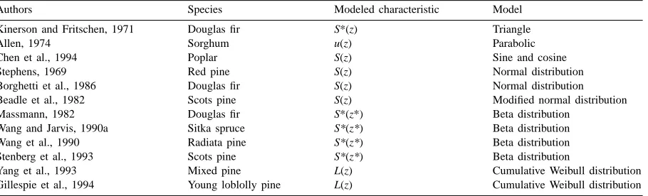
As an example, Fig. 1 expresses the dynamics of the probability density of the stem height zP and its
fitting by the normal distribution fzP(zP). At the
be-ginning of the vegetation period, data are sufficiently well described by the normal distribution. In the sec-ond half of summer, however, stems can be classified into two hierarchical categories — fast growing and suppressed stems. The height distribution function be-comes bimodal. During the following years of growth (Ross and Ross, 1998) this tendency becomes even more pronounced.
Table 2 presents the values of the parameters of the normal distribution during the growth period of 1998. They increase monotonically with time and are fitted by the third order polynomials as a function of time:
hzP(t )i =0.61+0.55t+2.49×10⁻²t2 −1.62×10⁻³t3, R2=0.99, σzp(t )= −4.62+1.22t−0.99×10⁻²t2+0.38
×10−2t3, R2=0.99. (9)
Time count in days (N) starts from 1 June.
On 23 November the distribution function fzP(zP)
Fig. 1. Probability histograms of the willow stem height zP (1zP=0.1 m) on 4 days through the growing season in 1998. f1 — height distribution of suppressed stems, f2 — height distribution of dominating stems, f1+f2 — superposition, f — all stems together.
Table 2
Dynamics of the parameters of the normal distribution — mean hzPi and standard deviation σzP — used for fitting the crown height distribution function fzP(zP) during the growing season in 1998a
Date N No obs. hzPi(m) σzP(m) R2
19 June 19 335 0.81 0.16 0.960
1 July 31 336 0.94 0.23 0.948
21 July 51 318 1.35 0.37 0.912
11 August 72 313 1.68 0.48 0.757
26 August 87 261 1.92 0.51 0.713
9 September 101 261 2.01 0.54 0.642 16 September 108 347 2.08 0.61 0.514 23 November 176 336 1.78 0.87 0.380
Suppressed I – – 1.33 0.47 –
Fast growth II – – 2.53 0.31 –
aN — number of days counted from 1 June.
It should be noted that since the role of suppressed shoots in the canopy’s radiative transfer processes as well as in photosynthesis and other processes is rather
small, then instead of bimodal height distribution, the averaged distribution as a rougher approximation can be used.
The top level of the canopy foliage zU(t) can be
considered as a random quantity. We will determine it by
zU(t )= hzP(t )i +2σzP(t ). (10)
The lower level of the canopy foliage, zL, increasing
monotonically with time, was fitted by
zL(t )=3.37×10⁻¹−1.29×10⁻²t
+1.42×10⁻⁴t2, R2=0.97 (11) Fig. 2 expresses the dynamics of some willow coppice parameters during the growth period of 1998.
Thus when one has fitting polynomials for the parameters of the normal distribution, hzP(t )i and
Fig. 2. Seasonal variation of some structural characteristics of the willow coppice during the growth period in 1998. LAI — Leaf Area Index, zU — upper level of the canopy foliage, zL — lower level of the canopy foliage.
fzP(zP, t) can be calculated for any day of the growth
period.
4.1.2. Correlation between stem foliage height and foliage area
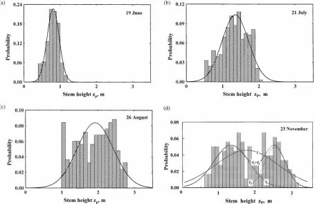
The correlation was estimated seven times during the growth period of 1998, R2 being between 0.89 and 0.98. In Fig. 3, as an example, the curves SP(zP)
express the correlation for June, August and October. During the growth period, b0and b change (Fig. 4)
and can be fitted by the polynomials
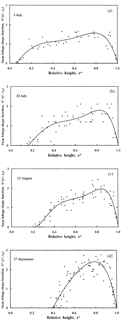
b0(t )=7.07×10⁻²−4.34×10⁻⁴t,
R2=0.94; (2a)
b(t )=3.44−2.48×10⁻²t+1.53×10⁻⁴t2,
R2=0.63. (3a)
Fig. 3. Willow stem foliage area SPvs stem height zP.
Fig. 4. Seasonal variation of the empirical coefficients b0 (a) and b (b) in Eq. (1).
By means of Eqs. (1), (2a) and (3a) we calculated stem foliage area for any height zP for any day.
4.1.3. Estimation of the shape function of stem foliage vertical distribution
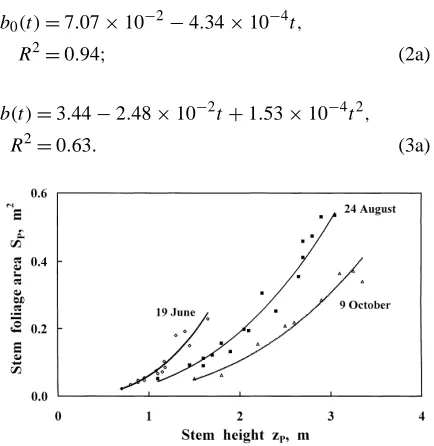
On sampling days tm, the leaf area in different
lay-ers of sample stems was measured, and S*(zi∗, tk) was
calculated using Eq. (6). As an example the values of S*(z∗i, tk) for four sampling days in different months
are presented in Fig. 5. Scattering of points character-izes the error made in determination of the shape func-tion. Typically, in midsummer months, a more rapid increase is seen in the shape function S*(z∗
i, tk) with
z*, starting from z*=0.6. This may be partly caused by the sprouting of small lateral branches on the stem and partly by fact that the largest leaves in the foliage layer are located within the relative height1z*=0.8−0.9.In accordance with Eq. (6b) S*(z∗n, tk) as the function of
the relative height zn∗ was approximated by the fifth order polynomials whose coefficients aikare given in
Fig. 5. Shape function S*(z*) of stem foliage vertical distribu-tion throughout the growth period in 1998. Points correspond to measured values, curves — to fitted polynomials.
The fitting polynomial corresponds to some ‘mean’ stem foliage vertical distribution averaged over the whole shoot height range. During the growth period, maximum leaf area density is located at z*=0.8, and the maximum value of S* fluctuates between 1.5 and 2.5.
Having a set of coefficients aikand applying Eq. (4)
to each day and each relative height z* it is possible to calculate the values of the shape function S*(z*, t).
4.1.4. Calculation of leaf area density and leaf area index
Finally, one can calculate the canopy leaf area density, u(z, t) as the function of height and time. In accordance with Eq. (8) the leaf area density u(z, t) is determined by three functions: distribution of stem height, interrelationship between stem height and stem total leaf area, and the shape function of stem foliage vertical distribution.
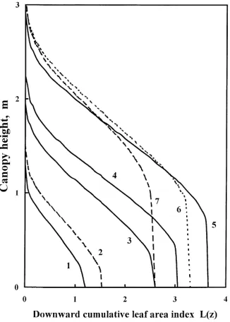
The downward cumulative leaf area index L(z), esti-mated for different days of the growth period, is given in Fig. 6.
5. Discussion
The presented interpolation method has several con-straints. In the first half of the growing season, stem height distribution was approximated by the normal distribution, sample size being 250–350 stems. How-ever, agreement was not the best (see Table 2). Conjec-turing that the sample size was too small, we doubled the number of samples during a special experiment, which still did not improve agreement essentially.
In the second half of the growing period, stem height distribution function has a tendency to transform from unimodal to bimodal. This is caused by competition between stems and by development of stem hierarchy (e.g. suppressed and dominant stems). As we have demonstrated earlier for the second year of growth, height distribution becomes bimodal and can be fitted by superposition of two normal distributions (Ross and Ross, 1998). Actually, the share of short stems in total canopy leaf area is not very large, and more careful fitting is essential in the range of long stems.
approx-Table 3
Empirical coefficients aik in Eq. (6b) for calculation of the shape function of the stem foliage vertical distribution S*(z∗n, t) at different relative heightsz∗
n z∗
n ai0 ai1 ai2 ai3 R2
0.9 −6.35×10⁻¹ 8.06×101 −1.1×10⁻³ 3.95×10⁻⁶ 0.894
0.8 6.55×10⁻¹ 4.09×10⁻² −4.76×10⁻⁴ 2.11×10⁻⁶ 0.975
0.7 1.45 −4.05×10⁻¹ 3.86×10⁻⁵ 1.43×10⁻⁶ 0.994
0.6 1.58 −1.66×10⁻² 3.00×10⁻⁴ −1.26×10⁻⁶ 0.997
0.5 1.53 −2.23×10⁻² 4.05×10⁻⁴ −2.50×10⁻⁶ 0.984
0.4 1.72 −3.33×10⁻² 5.71×10⁻⁴ −3.44×10⁻⁶ 0.992
0.3 6.56×10⁻¹ 3.24×10⁻² −7.82×10⁻⁴ 3.88×10⁻⁶ 0.981
0.2 2.85 −9.14×10⁻² 9.63×10⁻⁴ −3.32×10⁻⁶ 0.999
imation (R2=0.86÷0.98) and the seasonal change of the empirical parameters b0 and b can be
success-fully fitted by polynomials, R2 being 0.94 and 0.89, respectively.
Estimation of the shape function of the vertical distribution of the stem foliage is less exact. When defining the shape function we assume that the shape function of the vertical distribution of the stem foliage is similar for all stems. However, this assumption is not exact for the second half of the growth period. Short branches with a length of 3–8 cm develop in the
Fig. 6. Downward cumulative leaf area index L(z) vs height on different days of the growth period in 1998. 1 — 25 June, 2 — 3 July, 3 — 15 July, 4 — 28 July, 5 — 28 August, 6 — 14 September, 7 — 7 October.
upper part of long stems causing additional increase in leaf area density at the relative height of about z*=0.7−0.9.
This may increase dispersion of the experimental points in Fig. 4. One source of errors is the limited number of sampled stems. Practically, we were able to measure leaf area distribution for 15–30 stems on sam-pling days, which should represent all height classes of zP. However, in radiative transfer and
photosynthe-sis, leaf area distribution in upper canopy layers plays a more important role and hence the share of dominant trees is larger.
The success of the method depends also on the fitting accuracy of the temporal course of model pa-rameters during the growing period. Increasing the number of sampling days improves the situation. Abnormal weather conditions (drought, late frosts, etc.) may affect leaf and shoot growth and cause a non-smooth change of model parameters. Under such conditions input parameters should be estimated at shorter intervals.
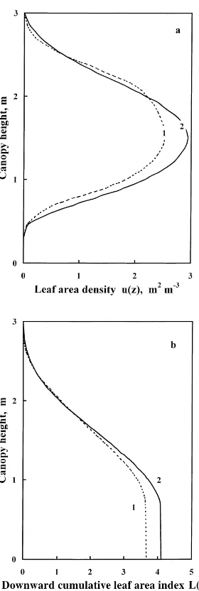
Fig. 7. Vertical distribution of (a) the leaf area density u(z) and (b) the downward cumulative leaf area index L(z) on 24 August 1998. 1 — experimental data, 2 — calculated using interpolation method.
6. Concluding remarks
Long-term calculation of canopy photosynthesis, transpiration, growth and other ecophysiological pro-cesses need a daily input parameter of the vertical dis-tribution of canopy leaf area. Its direct measurement is very tedious and time consuming and therefore cor-responding phytometrical measurements are usually carried out after 15–20 days.
This paper presents a statistical interpolation method which allows calculation of the function u(z) as well as the downward cumulative leaf area index L(z) and the leaf area index LAI for every day dur-ing the growth period when necessary phytometrical measurements are performed on sampling days. The method is based on the estimation of three statistical phytometrical functions: (i) probability density func-tion of stem height, (ii) interrelafunc-tionship between stem height and stem foliage area, and (iii) shape function of stem foliage vertical distribution. The method was applied for willow coppice in Estonia in the growth period of 1998.
Due to the great variability of the canopy leaf area density u(z), the error of our method has been estimated at about 10–15%. Among different input functions the greatest error is caused by the shape function of stem foliage vertical distribution. Increas-ing the number of samplIncreas-ing days durIncreas-ing the growth period the error of method decreases. The method uses time fitting polynomials up to the fifth order, which does not present a problem for a PC owner.
To our knowledge, the present study is the first at-tempt to elaborate a statistical interpolation method to be used for calculation of plant canopy foliage area and its vertical distribution for any day of the growing season.
The results of the study can be employed as the input parameters of comprehensive models of canopy photosynthesis and productivity. The applicability of the method for other plant canopy types needs further research.
7. List of symbols
b0(t) empirical constant (m)
b(t) empirical constant (–)
fzP(zP, t) stem height probability density
distribution function L(z, t) downward cumulative leaf
area index (m2m−2)
LAI(t) leaf area index (m2m−2)
N number of days counted from
1 June (day)
NP stem density (stem m−2)
area of individual stem (m2m−1per stem)
SP(zP) total leaf area of individual stem
at height zpin m2(m2per stem)
S∗(z∗)=SPzPS(z) shape function of the vertical distribution of the stem foliage (–)
u(z,t) single side leaf area density (m2m−3)
zL bottom level of canopy foliage
(m)
zP stem height (m)
hzP(t )i mean stem height (m)
zU top level of canopy foliage (m)
z*=z/zP relative height (–)
z∗L=zL/zP relative bottom level of canopy
foliage (–)
σzP(t) standard deviation of stem
height (–)
Acknowledgements
The research was supported by the ESF Grant No. 2668. The authors thank Mrs. Eneken-Mall Ross for assistance in fieldwork and data processing, Mrs. Viivi Randmets for technical aid, Mrs. Ester Jaigma for revision of the English text and Dr. Madis Sulev and Matti Mõttus for useful comments. The regional edi-tor of the journal Dr. J.B. Stewart and the anonymous reviewers are highly acknowledged for their com-ments and suggestions in improving the manuscript.
References
Allen Jr., L.J., 1974. Model of light penetration into a wide-row crop. Agron. J. 66, 41–47.
Beadle, C.L., Talbot, H., Jarvis, P.G., 1982. Canopy structure and leaf area index in a mature scots pine forest. Forestry 55, 105– 123.
Borghetti, M., Vendramin, G.G., Giannini, R., 1986. Specific leaf area and leaf area index distribution in a young Douglas-fir plantation. Can. J. For. Res. 15, 1283–1288.
Cescatti, A., 1997a. Modelling the radiative transfer in discontinuous canopies of asymmetric crowns I. Model structure and algorithms. Ecol. Model. 101, 263–274.
Cescatti, A., 1997b. Modelling the radiative transfer in discontinuous canopies of asymmetric crowns II. Model testing and applications in a Norway spruce stand. Ecol. Model. 101, 275–284.
Chen, S.G., Shao, B.Y., Impens, I., Ceulemans, R., 1994. Effects of plant canopy structure on light interception and photosynthesis. J. Quant. Spectrosc. 52, 115–123.
Gillespie, A.R., Allen, H.L., Vose, J.M., 1994. Amount and vertical distribution of foliage of young loblolly pine trees as affected by canopy position and silvicultural treatment. Can. J. For. Res. 24, 1337–1344.
Kinerson, R., Fritschen, J.L., 1971. Model in a coniferous forest canopy. Agric. Meteorol. 8, 439–445.
Koppel, A., Perrtu, K., Ross, J., 1996. Estonian energy forest plantations — general information. In: Perttu, K., Koppel, A., (Eds.), Short Rotation Willow Coppice for Renewable Energy and Improved Environment. Proc. joint Swedish–Estonian seminar, 24–26 September 1995. Swedish Univ. Agric. Sci. Uppsala, Report 57, pp. 15–24.
Massmann, W.J., 1982. Foliage distribution in old-growth coniferous tree canopies. Can. J. For. Res. 12, 10–17. Ross, J., 1981. The Radiation Regime and Architecture of Plant
Stands. Dr. W. Junk Publishers, The Hague, Boston, London. Ross, J., Ross, V., 1969. Vertical distribution of leaf area in crop
stands. Photosynthetic Productivity of Plant Stand. Acad. Sci. ESSR, Inst. Phys. Astron. Tartu, 83–01. (in Russian, in English see Ross, 1981)
Ross, J., Ross, V., 1996a. Leaf and stem area and their vertical distribution in willow stands. In: Perttu, K., Koppel, A. (Eds.), Short Rotation Willow Coppice for Renewable Energy and Improved Environment. Proc. joint Swedish-Estonian seminar, 24–26 September 1995. Swedish Univ. Agric. Sci. Uppsala, Report 57, pp. 33–50.
Ross, J., Ross, V., 1996b. Phytometrical characteristics of the willow plantation at Tõravere. In: Perttu, K., Koppel, A. (Eds.), Short Rotation Willow Coppice for Renewable Energy and Improved Environment. Proc. joint Swedish–Estonian seminar, 24–26 September 1995. Swedish Univ. Agric. Sci. Uppsala, Report 57, pp. 133–145.
Ross, J., Ross, V., 1998. Statistical description of the architecture of a fast growing willow coppice. Agric. For. Meteorol. 91, 23–37.
Stenberg, P., Smolander, H., Kellomäki, S., 1993. Description of crown structure for light interception models: angular and spatial distribution of shoots in young Scots pine. Studia Forestalia Suecica 191, 43–50.
Stephens, G.R., 1969. Productivity of red pine 1. Foliage distribution in tree crown and stand canopy. Agric. Meteorol. 6, 275–282.
Wang, Y.P., Jarvis, P.G., 1990a. Description and validation of an array model — MAESTRO. Agric. For. Meteorol. 51, 257–280. Wang, Y.P., Jarvis, P.G., 1990b. Influence of crown structural properties on PAR absorption, photosynthesis and transpiration in Sitka spruce: application of a model (MAESTRO). Tree Physiol. 7, 257–316.
Wang, Y.P., Jarvis, P.G., Benson, M.L., 1990. Two-dimensional needle area density distribution within the crowns of Pinus radiata trees. For Ecol. Manage 32, 217–237.