KILIMANJARO ICE CLIFF MONITORING WITH CLOSE RANGE
PHOTOGRAMMETRY
Michael Winkler a, W. Tad Pfeffer b, Klaus Hanke c
a Center of Climate & Cryosphere, Department of Meteorology and Geophysics, University of Innsbruck, Austria (michael.winkler@uibk.ac.at) b INSTAAR, Univ. of Colorado, Boulder, CO, USA (tad.pfeffer@colorado.edu)
c Surveying and Geoinformation Unit, Institute for Basic Sciences in Civil Engineering, University of Innsbruck, Austria (klaus.hanke@uibk.ac.at)
Commission V, WG V/6
KEY WORDS: Monitoring, Kilimanjaro, Glacier, Climate Change, Close Range Photogrammetry
ABSTRACT:
The glaciers on the summit plateau of Kibo, the main peak of the Kilimanjaro massif (3°S, 37°E, 5895 m a.s.l.) in Tanzania, are characterized by steep ice cliffs at their margins. These form-persistent cliffs continuously retreat and, consequently, govern the decrease in plateau glacier area. In order to quantify the ice cliff recession and study their morphology, close-range terrestrial photogrammetry combined with automatic stereo matching techniques was used to derive high resolution digital surface models of a south-facing “sample cliff” at four different dates. Results confirm, firstly, the annually bimodal nature of the recession being 15 cm/month during a 4.5 month sunlit phase and 2 cm/month during the remaining 7.5 month shaded phase, and, secondly, the tendency towards an “ideal cliff orientation”, which is either south- or north-facing and about 70°-75° steep. Moreover, the hypothesis of a predefined decay period for the plateau ice is supported by this study and it is shown that terrestrial photogrammetry is not only cheap and lightweight but also very suitable for ice surveys at the decameter scale.
1. INTRODUCTION
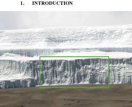
Figure 1: A part of the Northern Ice Field on Kibo. The “sample cliff” is outlined by the green rectangular.
The Kilimanjaro massif in Tanzania, East Africa, consists of three volcanic mountains: Shira, Mawenzi, and Kibo, the highest peak of Africa (5895 m a.s.l.) and well known for the glaciers atop it. These glaciers have been investigated since explorers first reached the crater rim (e.g. Meyer, 1891). For glaciological process studies, it is necessary to distinguish between the nearly horizontal surfaces of the summit plateau glaciers, the steep glaciers on the slopes below the summit, and the land-based ice cliffs at the summit glacier margins (cf. Kaser et al., 2004, and Cullen et al., 2006), as these contrasting ice surfaces are governed by different micro-meteorological conditions. The aggregate glacier area (1.85 km² in 2007 according to Thompson et al., 2009) has been decreasing since
the late 19th century (Osmaston, 1989) and, undoubtedly, this is closely linked to the recession of the ice cliffs (e.g. Winkler et al., 2010). The existence and the form-persistence of the ice cliffs is an essential prerequisite for the recently presented hypothesis of a 165 years decay period for the plateau ice from a maximum extent to disappearance (Kaser et al., 2010). The study in hand quantifies the rate of the recession of the ice cliffs, and analyses the tendency for the cliffs to maintain their form, on the basis of four consecutive terrestrial photogrammetric surveys at the highest-ever temporal and spatial resolution and presents an outstanding application of this method at that scale in glaciological studies.
A section of the land-based marginal ice cliff of the Northern Ice Field was chosen for the surveys, hereafter called “sample cliff” (Figure 1). It is situated at 5760 m a.s.l., 03°03.60’ S, 37°20.94’ E, and spans ca. 65 x 25 m. The cliff surface faces approximately south, consists of very pure, high-albedo ice and is shaped by elongated near-vertical features like pillars, dihedrals, and ramps as well as smooth parts (see Winkler et al. (2010), where the sample cliff is defined in a similar way). The reason for the choice of the sample cliff was threefold: it is characteristic for most of the cliffed margins in terms of height, structure, and setting; an automatic weather station has been operating at its base since 2005; and unpublished surveys with a total station were carried out there on September 16-18, 2004 and on January 18-19, 2006 by W. J. Duane (personal communication, 2008 and 2011). Due to the lack of absolute reference systems, quantitative comparisons of those surveys with the results of the current study are impossible, but qualitative comparison proves that the aspect and slope of the sample cliff have not changed significantly since 2004.
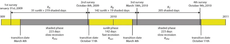
Winkler et al. (2010) illustrated that the recession of the ice cliffs is bimodal over the course of the year due to changing incident solar radiation at the cliff surfaces. Transition dates between the two phases (Figure 2) were defined using a solar
radiation model. Slow recession rates occur during the 7.5 months of the “shaded phase” (ca. March 4 to October 11) when sublimation is the only possible ablation process. Fast recession rates are measured during the remaining 4.5 months
of the “sunlit phase”, when enough solar energy is available to raise the cliff surface temperature to 0°C and to allow melting during some hours of the days.
Figure 2: Sequence of sunlit and shaded phases as well as of survey dates at the sample cliff. The given amounts of days are approximate values and underlie small interannual variations. See text for elucidations.
2. METHODS
2.1 Photogrammetric surveys
The first photogrammetric survey of the sample cliff was accomplished on January 31, 2009. A Nikon D2X DSLR camera (12.4 megapixels) mounted on a standard tripod and photogrammetrically calibrated lenses with fixed focal lengths of 20 mm and 28 mm were used. After some tests, landscape oriented photos with the 20 mm lens and an object distance of approximately 40 - 80 m provided the optimal coverage for the area of interest. The photos could only be taken from the ash ground in front of the cliff (not from any elevated position) and the exterior orientation of the camera stands (position and direction) was not measured.
Five reference targets (Styrofoam™ and tennis balls) were permanently marked with spikes anchored in the ash ground; two more were placed on the automatic weather station which was not moved between two consecutive surveys. Another eight temporary reference points were put on the ash ground and four were placed up on the edge of the ice cliff (see Winkler et al., 2010, for details). A Leica TCRA 1101 total station was used to define a local coordinate system and to survey all 19 reference points. A total of ca. 170 photos were taken with different settings and finally 17 photos proved to be sufficient to build a photogrammetric model using the software PhotoModeler® Scanner (Hullo et al., 2009) that included all reference points. The total station coordinates of three of the permanently marked points were used to scale and orient (= exterior orientation) the model in space. As a last step three optimal photo pairs were chosen, based on PhotoModeler® Scanner’s quality assessment report, to derive a dense surface mesh of the sample cliff by automatic stereo matching techniques (Hullo et al., 2009; Remondino and El-Hakim, 2006). After some rather time-consuming tuning of the meshing parameters, the method worked surprisingly well for this ice surface.
The second survey was made on October 8, 2009, close to the transition date from the shaded to the sunlit phase (Figure 2). The procedure was essentially the same as 250 days before but this time no total station was used, with the result that the survey equipment had a total weight below 10kg. A Nikon D200 DSLR camera (10.2 megapixels) with a calibrated fixed focal length 20 mm lens was used and two additional reference points were permanently marked with spikes. As there was no tachymetric survey made, a tape measure was used to measure the distances between the reference points in order to get an independent estimate of their precision in the photogrammetric model. The model itself was built from 19 photos and transformed into the stationary reference system of the first
survey by using the same three surveyed fix points for scale and rotation. A detailed description of this survey campaign is given by Winkler et al., 2010.
The third and the fourth photogrammetric surveys were accomplished on March 18, 2010 and October 9, 2010, respectively, again close to the transition dates between the two recession phases, and no further changes were made in the procedure compared to the second campaign. 26 and 15 photos were used to build the models, respectively.
2.2 Data processing
The resulting point clouds of the surface meshes calculated by PhotoModeler® Scanner contained little noise for all four dates. Outlier points (< 5 % of all points) were eliminated manually. Finally, a mean point cloud resolution of between 618 and 828 points per square meter cliff face area was achieved, depending on the surveying date.
The coordinate system was initially defined by East, North, and Up. To make analyses easier, the point clouds were transferred to a local coordinate system with the x-axis parallel to the mean cliff base, the y-axis vertical and the z-axis orthogonal to x and y. The transferred point clouds were converted to regular gridded digital surface models (DSMs). A grid size of 25 cm turned out to be the best compromise between retaining information about small scale features and deriving robust DSMs for the following analyses. Thus, averaged over all four DSMs each grid cell is represented by 44 ± 26 points.
With the z-axis defined perpendicular to the cliff face, i.e. in the main direction of the recession, the difference in z between the individual grid cells of different DSMs can directly be interpreted as recession (or advance) at the respective grid cell location. From the four surveys, three recession periods, A, B, and C were analyzed on basis of the exact dates of the surveys and the transitions between the phases (Figure 2). The respective amounts of the recessions, RA, RB, and RC are
sun recession rates for the sunlit and the shaded phase and recession maps for each phase can be derived (Figure 3). In addition,
maps showing slope and aspect at the 25 x 25 cm resolution were produced (Figure 4).
2.3 Precision
The precision of the cliff surface models was estimated using intrinsic PhotoModeler® Scanner parameters as well as the extrinsic, independent methods of tape measurements and DSM intercomparison. The maximum point residual of all the
photogrammetric models was below 1.5 pixels and the mean tightness of the reference points was ca. 3 cm, with no value higher than 5 cm (point residuals and tightness are parameters provided by PhotoModeler® Scanner’s project quality reports). The tape measurements between the reference points differ in a range of ~5 cm (~0.2-0.5 %) from the photogrammetric solution, as does the deviation between the first photogrammetric model and the tachymetric model.
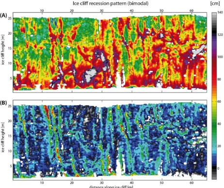
Figure 3: Ice cliff recession at the sample cliff in centimeters: (A) during the “sunlit phase” (ca. October 12 to March 3) with a mean recession of 15 cm/month, (B) during the “shaded phase” (rest of the year) with a mean rate of 2 cm/month. The resolution in width
and height is 25 cm. The precision of the method is given in the text.
Unfortunately, PhotoModeler® Scanner does not provide parameters describing the precision of the dense surface meshes created by automatic stereo matching. In order to derive an estimation of that, three additional surface meshes were calculated for the first survey using different photo pairs for stereo matching. The resultant point clouds were used to derive three more raster DSMs with 25 x 25 cm grid size. Together with the initial DSM (see section 2.1.) these provide a batch of four DSMs for the first survey, all of which were derived by matching different photo pairs. As expected, all the DSMs had “holes” at different locations but for more than 4000 grid cells z-values were available for at least two of the DSMs. The standard deviations of the z-values of those cells were
calculated: for 64 % of the cells it was below 10 cm, the median of the standard deviations was 7.7 cm.
This result suggests that the error in the DSMs is mostly due to the error in the automatic stereo matching procedure because the precision of the reference points is better (ca. 5 cm, see above). However, according to A. Walford (Eos Systems Inc. CEO and developer of PhotoModeler® Scanner; personal communication, 2011) the precision of the dense surface meshes in the z-direction should be similar to the reference point precision multiplied by the so-called downsampling factor, which is used during the meshing procedure, or up to 10-times better. In the worst case, this would lead to a precision of the surface meshes produced during this study of 6.5, 3.5, 4.5, and 3.0 cm, respectively. The smoothness of the point cloud
surfaces furthermore suggests that the point-to-point precision is actually at the order of a few centimeters.
Taking the conservative assumption that the z-value precision of each single grid cell of the derived DSMs is 7.7 cm, which is
the median value from our DSM comparison, the precision of the derived recession between two surveys is 11 cm.
Figure 4: Ice cliff aspect and slope in October 2010. On average the ice cliff faces approximately south (173° from north) and its slope is 66.9° with only minor changes occurring over time. The resolution in width and height is 25 cm.
3. RESULTS
In its entirety, aspect and slope of the sample cliff are 173° (from north) and 66.9°, respectively, with only small variations during the course of the four surveys (2.6° and 1.0°, respectively). The deviation in aspect from that given in Winkler et al. (2010) is due to the slightly different, more representative, delimitation of the sample cliff in the current study. The cliff height was ca. 25 m for all four surveys, with no significant changes in between. Undoubtedly, the most notable change occurring at the sample cliff is its recession. The differences between the photogrammetrically-derived DSMs confirm the point measurements of the recession presented by Winkler et al. (2010) in the matter of magnitude and annual bimodality. In addition, areal pictures of the recession as well as of aspect and slope are now available at high resolution and on a sub-annual timescale (Figs. 3 and 4).
The recession pattern during the “sunlit phase” (142 days) is illustrated in Figure 3A. The cliff receded at an average rate of 69 cm per sunlit phase which equates to 15 cm/month. Significant advances can only be detected at the very bottom of the cliff where porous cones of ice develop from grains that fall off the cliff surface due to melt processes (see Winkler et al., 2010). These cones, in turn, disappear during the “shaded phase” when no melting and grain fall-off support cone growth, but when the ash ground still gets warmed by direct sunlit and heat conduction melts away the deposits. In general, during the shaded phase, recession is much smaller than during the sunlit phase (Figure 3B), except for some areas along linear features like pillars and grooves and at the former spots of the now melted cones. This adds up to a cliff-wide average recession of 15 cm during the 223 days of the shaded phase which equates to 2 cm/month. Recession during the sunlit phase is 7.5-times faster than during the shaded phase.
Maps of aspect and slope (for October 2010) are plotted in Figure 4. The linear features of the cliff mentioned above are distinctly resolved in the aspect map (upper panel of Figure 4). The alternation of pillars and grooves cause a periodic change of east- and west-facing bands along some sections of the ice cliff denoted by bluish-gray and reddish stripes in Figure 4. These areas coincide with the areas with high recession during the shaded phase (Figure 3B). This will be referred as “coincident ASPECT-SHADED” in the following.
The slope map (lower panel of Figure 4) shows the distribution of structures such as ledges and ramps, where the surface slope is less than the predominant steepness. The recession map of the sunlit phase (Figure 3A) shows that the highest recession rates occur on those parts of the sample cliff with lower slope angles. This is referred to as “coincident SLOPE-SUNLIT”.
Figure 5: The tendency of the ice cliff to form and to maintain an “ideal orientation”, which is assumed to be near-vertical and
south-facing.
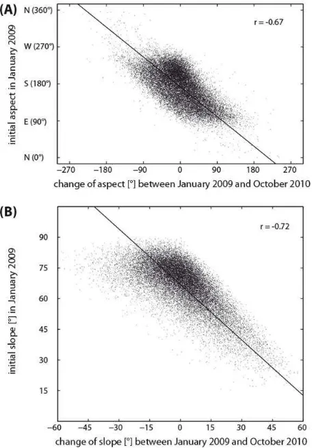
The reasons for the coincidences “ASPECT-SHADED” and “SLOPE-SUNLIT” become clear when looking at the scatter plots in Figure 5. The aspects of the individual grid cells of the initial survey from January 2009 are plotted versus the respective changes in aspect compared to the last survey from October 2010 (Figure 5A). There is a tendency (r = -0.67) for initially east- or west-facing areas to turn about a vertical axis to become “more south-facing” 20.5 months later. The average aspect, 173° from north, seems to be close to the “ideal aspect” of the cliff, which presumably is south. This result impressively confirms the findings of e.g. Winkler et al. (2010) who state that east- and west-facing marginal cliffs at Kibo’s ice bodies on the whole are rare compared to poleward-facing cliffs because they
receive too much energy from the sun and tend to melt away. Further, the finding strengthens the hypothesis of persistent ice cliffs controlling an incessant shrinkage of the horizontally projected surface area of the plateau ice (Kaser et al, 2010). The few existing east- or west-facing cliffs are characterized by rough, lamella-like surfaces where, after closer consideration, the main portion is either north- or south-facing (Winkler et al., 2010).
The scatter plot in Figure 5B shows a similar picture for slope as Figure 5A does for the aspect. Cliff areas flatter than the mean cliff slope steepened up to ca. 70°-75° and areas that were already close to the mean slope angle at the first survey remained mainly unchanged (r = -0.72). Some initially steep parts also flattened (which is investigated in the next paragraph) but in general there is a tendency towards slopes of roughly 70°-75°, presumably the “ideal cliff slope”.
The aforementioned tendencies towards an “ideal” ice cliff orientation and steepness raises the question of why deviations manifested as e.g. pillars, dihedrals, ramps, and ledges appear at all. The answer to that is found in the existence of (1) small impurities in the ice that lower local albedo and cause differential ablation at particular spots, and (2) meltwater running or trickling down the cliff during the sunlit phase, which on the one hand erodes the surface, and on the other hand can also refreeze to form irregularities such as icicles (Uhlig, 1908; Jäger, 1931; Winkler et al., 2010).
4. DISCUSSION AND OUTLOOK
Close-range terrestrial photogrammetry was used to derive digital surface models of a land-based marginal ice cliff on Kilimanjaro at four different dates. The chosen 1750 m² “sample cliff” (Figure 1) is situated at the southern margin of the Northern Ice Field on Kibo, the only glaciated peak of Kilimanjaro, at 5760 m a.s.l. Except for the first survey, when a total station was used to construct a reference system, the photogrammetry equipment only consisted of a DSLR camera on a tripod, a calibrated, fixed focal length 20 mm lens, 19 styrofoam and tennis balls used as reference points, a 50 m tape measure, and 7 steel spikes for permanent marking. With this low-cost and lightweight equipment a referencing tightness of ca. 3 cm and reference point residuals <1.5 pixels could be achieved using the photogrammetric software PhotoModeler® Scanner. The texture of the ice cliff surface turned out to be very suitable for automatic stereo matching techniques and, after having derived 25 x 25 cm gridded data sets from the point clouds, the average precision of each individual grid cell was estimated to be 7.7 cm.
The most remarkable change happening at the cliff is its bimodal recession. During 4.5 months (mid-October to begin of March) when solar radiation at the cliff surface is high, the sample cliff recedes at a mean rate of 15 cm/months (Figure 3A). During the remaining 7.5 months of the year the recession rate is decreased to 2 cm/month (Figure 3B). Of course, the recession measured by photogrammetry cannot be interpreted offhand as the (negative) surface mass balance at the ice cliff without investigating possible deformation. However, Kaser et al. (2004) and Winkler et al. (2010) attest that ice flow on the plateau glaciers of Kibo is of only minor importance because the ice is too thin and there is no evident sign of deformation at the margins. Preliminary modelling results (G. H. Gudmunsson and A. H. Jarosch, both personal communication, 2008 and 2010, respectively) show maximum deformation rates at the
order of a few centimeters per year but more work needs to be done on this issue.
Assuming that the ice flow component can be neglected, the annual recession rate at the sample cliff of ca. 84 cm equates to a mass loss of ca. 760 kg/m² averaged over the sample cliff area (taking 900 kg/m³ for the ice density). This clearly contrasts with the mean annual net surface mass balance between the times of the first and the last photogrammetric survey at some places of the gently inclined plateau glacier surfaces. For example, at an automatic weather station, which is mounted about 2 km south of the sample cliff at the upper end of Kersten Glacier (see e.g. Mölg et al., 2009), ca. +150 kg/m² of mass gain was measured during the respective period. This supports the findings presented by Kaser et al. (2010) who outline the great importance of the ice cliffs for mass balance and glacier area assessments on Kibo.
There is a tendency towards an “ideal” cliff orientation which confirms former results of e.g. Winkler et al. (2010), expressing why there are virtually no east- and west-facing cliffs as well as no gently sloped ice surfaces on the crater plateau. This characteristic of the cliffs to preserve slope and orientation strongly supports the hypothesis of short lived plateau ice on Kibo (Kaser et al., 2010) which excludes a long lasting history such as suggested by Thompson et al. (2002). The sample cliff’s average aspect and slope (173° from north and 66.9°, respectively) turn out to be close to the ideal, suggesting that this cliff will maintain its current orientation and slope in the future.
In principal, all the results from the south-facing sample cliff are transferable to all other land-based ice cliffs on the plateau glaciers of Kibo - including the north-facing ones - because the micro-climatological setting is the same for all of them. However, there might be some restrictions in assigning the results to ice cliffs that occur on top of the Northern Ice Field, which have ice surfaces at their base (Figure 1). The physical processes at these cliff faces might be different compared to those at the cliffs that have ash surfaces at their base. The drivers for the ice cliff recession have been partially discussed in Kaser et al. (2004, 2010) and Winkler et al. (2010). Ongoing analyses of energy balance data recorded from the Kibo ice cliff are expected to provide further insight into the processes that form and maintain the cliffs, and drive their recession.
ACKNOWLEDGEMENTS
This study was funded by the Austrian Science Fund FWF (grants P20089-N10 and P22106-N21). We want to thank the Tropical Glaciology Group from the University of Innsbruck and other colleagues for their valuable contributions during both, field and data work, especially G. Kaser, T. Mölg, L. Nicholson, R. Prinz, N.J. Cullen, M. Kaser, G. Neuerer, and C. “Lenz” Gratzer. We very much appreciate the excellent assistance of the Marangu Hotel, Moshi, TZ, and of all the guides and porters who helped us during our high altitude field works. Local support was given by the Tanzanian Meteorological Agency (TMA; with special thanks to Tharsis Hyera), the Commission of Science and Technology (COSTECH), the Tanzanian and Kilimanjaro National Park Authorities (TANAPA and KINAPA), and the Tanzanian Wildlife Research Institute (TAWIRI).
REFERENCES
Cullen, N.J., T. Mölg, G. Kaser, K. Hussein, K. Steffen, and D.R. Hardy (2006): Kilimanjaro Glaciers: Recent areal glacier extent from satellite data and new interpretation of observed 20th century retreat rates. Geophysical Research Letters, 33, L16502, doi:10.1029/2006GL027084.
Hullo, J.F., Grussenmeyer, P., and Fares, S. (2009): Photogrammetry and Dense Stereo Matching Approach Applied to the Documentation of the Cultural Heritage Site of Kilwa (Saudi Arabia). XXII CIPA Symposium (pp. 1-6). Retrieved from http://www.photomodeler.com/applications/articles_and_ reports.htm.
Kaser, G., D.R. Hardy, T. Mölg, R.S. Bradley, and T.M. Hyera (2004): Modern glacier retreat on Kilimanjaro as evidence of climate change: Observations and facts. International Journal of Climatology, 24, 329-339, doi: 10.1002/joc.1008.
Kaser, G., T. Mölg, N.J. Cullen, D.R. Hardy, and M. Winkler (2010): Is the decline of ice on Kilimanjaro unprecedented in the Holocene? The Holocene, 20, 1079-1091.
Jäger, F. (1931): Veränderungen der Kilimanjaro-Gletscher. In: Zeitschrift für Gletscherkunde XIX, 285–299.
Meyer, H. (1891): Zur Kenntnis von Eis und Schnee des Kilimandscharo. In: Petermanns Geographische Mitteilungen 36, 289–294.
Mölg, T., N.J. Cullen, D.R. Hardy, M. Winkler, and G. Kaser (2009): Quantifying climate change in the tropical mid troposphere over East Africa from glacier shrinkage on Kilimanjaro. Journal of Climate, 22, 4162-4181.
Osmaston, H. (1989): Glaciers, glaciations and equilibrium line altitudes on Kilimanjaro. In: Mahaney W. C. (ed.): Quaternary and environmental research on East African mountains. Rotterdam, 7–30.
Remondino, F., El-Hakim, S. (2006): Image-based 3D modelling: a review. Photogrammetric Record, 21(115), pp. 269-291.
Thompson, L. G.; Brecher, H. H.; Mosley-Thompson, E.; Hardy, D. R. and Mark, B.G. (2009): Glacier loss on Kilimanjaro continues unabated. In: Proceedings of the National Academy of Sciences 106 (47), 19770–19775.
Thompson, L. G.; Mosley-Thompson, E.; Davis, M. E.; Henderson, K. A.; Brecher, H. H.; Zagorodnov, V. S.; Mashiotta, T. A.; Lin, P.; Mikhalenko, V. N.; Hardy, D.R.; Beer, J. (2002): Kilimanjaro ice core records: Evidence of Holocene climate change in tropical Africa. Science 298: 589– 593.
Uhlig, C. (1908): Ostafrikanische Expedition der Otto Winter Stiftung. In: Zeitschrift der Gesellschaft für Erdkunde zu Berlin. 75-94.
Winkler, M., G. Kaser, N.J. Cullen, T. Mölg, D.R. Hardy, and W.T. Pfeffer (2010): Land-based marginal ice cliffs: focus on Kilimanjaro. Erdkunde, 64, 2, 179-193.