FEATURE MODELLING OF HIGH RESOLUTION REMOTE SENSING IMAGES
CONSIDERING SPATIAL AUTOCORRELATION
Y. X. Chen a , K. Qin a, *, Y. Liu b, S. Z. Gan a, Y. Zhan a
a School of Remote Sensing and Information Engineering, Wuhan University, Wuhan, China
b Information Technology Simulation Teaching and Research Section, Institute of Chemical Defense of CPLA, Beijing, China
Commission III, ICWG III/VII
KEY WORDS: high resolution, feature, modelling, spatial autocorrelation, segmentation
ABSTRACT:
To deal with the problem of spectral variability in high resolution satellite images, this paper focuses on the analysis and modelling of spatial autocorrelation feature. The semivariograms are used to model spatial variability of typical object classes while Getis statistic is used for the analysis of local spatial autocorrelation within the neighbourhood window determined by the range information of the semivariograms. Two segmentation experiments are conducted via the Fuzzy C-Means (FCM) algorithm which incorporates both spatial autocorrelation features and spectral features, and the experimental results show that spatial autocorrelation features can effectively improve the segmentation quality of high resolution satellite images.
* Corresponding author:E-mail address: qink@whu.edu.cn
1. INTRODUCTION
High spatial resolution remote sensing imagery obtained from satellite (IKNOS, Quickbird, GeoEye-1, WorldView-2, etc) and airborne sensors have become increasingly available in recent years (Johnson & Xie, 2011). These data provide amazing details of the Earth’s surface, but for information extraction from complex scene such as urban environment, it is difficult to obtain satisfactory results using only spectral information (Byun et al., 2011).
It is well known that combining spatial and spectral information is a good strategy to improve urban land use classification. Features extracted by using co-occurrence matrices, Gabor wavelets, morphological profiles, and Markov random fields have been widely used in the literature to model spatial information in neighborhoods of pixels (Akcay & Aksoy, 2008).
Spatial autocorrelation as spatial information is an inherent feature of remote sensing data and a reliable indicator of statistical separability between spatial objects. In remote sensing,spatial autocorrelation means the spectral dependence existing between a pixel and its neighbors, that is, spectral value of a pixel is usually not independent but correlated with those of its neighboring ones. Spatial autocorrelation provides us the structural information between spectral values of pixels, which is usually more stable and robust to noise than individual pixel. This information may be used to improve the segmentation quality or classification accuracy for spectrally heterogeneous classes and overcome the current spectral limitations of very high spatial resolution satellite images.
The basic approach modelling spatial autocorrelation is to use spatial autocorrelation statistics, including global statistics and local statistics. Global statistics of spatial autocorrelation such as Moran’s I and Geary’s C, are simple summary measures which are difficult to uncover the local spatial variability. Getis
statistic (Ord & Getis, 1995) is a measure of local spatial autocorrelation, which is quite effective in distinguishing “hot spots” and “cold spots”. Thus, it could be used, for example, to identify a group of bright or dark pixels that represent a spectral response from a homogeneous feature (Myint et al., 2007). Another approach modelling spatial autocorrelation is semivariogram, which is a geostatistical function and can be used to model spatial variation patterns of typical object classes in the image, providing structure information of spatial autocorrelation. The range of the semivariogram can be used as a measure of spatial dependency or homogeneity (Franklin et al., 1996) and it has been proved to be directly related to the size of objects or patterns in an image (Balaguer et al., 2010). Therefore, it may be used to determine the proper window size for each pixel in local spatial autocorrelation analysis.
This paper focuses on the analysis and modelling of spatial autocorrelation features for improving the segmentation quality of high resolution satellite images. The semivariograms are used to model spatial variability of typical object classes, while Getis statistic is used to calculate the local spatial autocorrelation based on range information provided by semivariograms. Two segmentation experiments based on Fuzzy C-Means (FCM) clustering algorithm (Bezdek, 1981) are conducted. The results show that spatial autocorrelation features can effectively improve the segmentation quality of high resolution satellite images.
2. STUDY AREA AND DATA
In this paper, the experimental data are Quickbird images of two different sites in Wuhan, China, with the resolution of panchromatic band 0.61 m and multi-spectral band 2.44 m. The image sizes of the two sites are 798 pixels×642 pixels and 349
pixels×220 pixels, respectively. In this paper, multi-spectral bands (band 4, band 3 and band 2) are used for experiments. The color images by fusing 4, 3, 2 bands are showed in Figure 1, and by field survey, the object classes of site 1 mainly include vegetation, waters, roads and ships, and in site 2, its typical object classes include buildings, shadows, vegetation and bare lands. Most of these object classes are spectrally heterogeneous in the images.
(a) site 1
(b) site 2
Figure 1. Quickbird color images of the study area
3. METHODOLOGY
3.1 Semivariogram
The semivariogram is a geostatistical function which describes the spatial variability of the values of a variable. The experimental semivariogram is defined as
2
where z (xi) is a regionalized variable, representing the value of the variable at the location xi . The lag h is the vector from pixel xi to pixel xi + h, and N (h) is the number of pixel pairs xi and xi + h.
Figure 2. Semivariogram and its parameters
Semivariogram has three basic parameters (Figure 2): nugget, sill and range. The nugget is an estimate of variance at distance (or lag) zero, which may be interpreted as a measure of variability inside the pixel cell. The semivariance is a function
of lag h, and the sill is the maximum semivariance level reached. The lag at which the sill reached is the range, which can be used as a measure of spatial dependency or homogeneity (Franklin et al., 1996) and it has been proved to be directly related to the size of objects or patterns in an image (Balaguer et al., 2010). In this paper, it is used to guide the selection of proper window sizes for local spatial autocorrelation analysis.
3.2 Getis statistic
Getis statistic is a local indicator describing spatial autocorrelation, which provides a measure of spatial dependence for each pixel. The standardized Getis statistic observation i, including i itself (i.e. wii=1), and zero otherwise;
are the mean and variance of values of all pixels, respectively.
Getis statistic describes the autocorrelation of a variable in a local region, and in particular, it is effective in identifying clusters of high values called “hot spots” or clusters of low values called “cold spots” in an image. In this paper, it is used to calculate the degree of local spatial autocorrelation.
3.3 Window determination by semivariogram and spatial
autocorrelation analysis by Getis statistic
Since Getis statistic is a function of distance d, it has the characteristics of scale. Therefore, one problem we have to deal with is how to select proper parameter d for local spatial autocorrelation analysis, which is also a problem determining proper window size (defined as (2d+1)*(2d+1)) for each pixel. We may take many different d values for repeated experiments, but it is time-consuming. Fortunately, the range of the semivariogram provides information about the length of spatial correlation in the images; pixels (or objects) separated by a distance less than the range are spatially correlated, whereas pixels at separations longer than the range are not (Meer, 2012).
To make full use of local spatial autocorrelation information, we limit window width (2d+1) not exceeding the maximum range of all the semivariograms characterizing all selected object classes, which could greatly reduce repeated experiments but also include autocorrelation information as much as possible within the window. In detail, we first select typical objects or their samples in the image and then modelled them by semivariograms. From semivariograms, the range of spatial variability of each object can be determined approximately by visual inspection (As window parameter d is a positive integer, approximate range values are enough for window determination). Then spatial autocorrelation degree is easily calculated using Getis statistic by equation (2) within neighborhood window (2d+1)*(2d+1). For each spectral band, spatial autocorrelation feature band can be obtained by assigning the value of spatial autocorrelation degree of each pixel to this pixel.
3.4 FCM clustering segmentation
For an image, clustering is a commonly used segmentation method, which usually employs spectral information of each pixel as feature vector and realize partition of the image in feature space by similarity measure.
As a generalization of classical k-means clustering, Fuzzy C-Means (FCM) algorithm is also a partition-based clustering method, which realizes the soft partition of a data set by minimizing the objective function (Bezdek, 1981)
2 following iterative formula (4) and (5)
2 number of clusters, N is the number of feature vectors, and m is
a fuzzy factor (m >1). Note that for
u
ki
{0,1}
, the Fuzzy C-Means (FCM) algorithm boils down to the hard c-means case (or classical k-means algorithm).For high resolution satellite images, clustering segmentation only using spectral information is difficult to obtain satisfactory results due to spectral variability. Spatial autocorrelation feature, as spatial information, may be incorporated into clustering segmentation algorithm to improve the segmentation quality.
In this paper, segmentation experiments are conducted via the Fuzzy C-Means (FCM) algorithm, which incorporates both spatial autocorrelation features and spectral features. The expected results are that spatial autocorrelation features can effectively improve the segmentation quality of high resolution satellite images.
4. RESULTS AND DISCUSSIONS
4.1 Semivariogram modelling
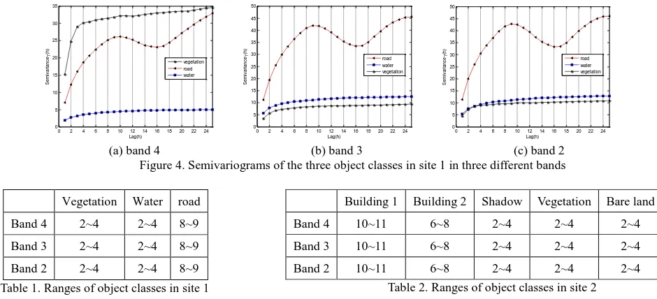
This paper first selects three typical object classes (figure 3) from the original image of site 1 (figure 1(a)): vegetation, water and road, but the other small objects like ships are not considered. The omni-directional semivariograms of theirs are calculated in three bands, respectively (figure 4).
(a) vegetation (b) water (c) road Figure 3. Typical object classes in site 1
From figure 4, we know different object classes correspond to different semivariograms, and thus they have different spatial variabilities. Semivariograms of water and vegetation are quite simple and similar except in band 4, and their ranges are all about between 2~4 pixels by visual inspection. Comparing with water and vegetation, semivariogram of the road is relatively complex, which is continuously fluctuant and unstable when lag h exceeds the range, implying that roads have more complex variation structure. The range of its semivariogram is about between 8~9 pixels. The detailed range information of the three object classes in site 1 is listed in table 1.
0 2 4 6 8 10 12 14 16 18 20 22 24 Figure 4. Semivariograms of the three object classes in site 1 in three different bands
Table 1. Ranges of object classes in site 1
This paper focuses on ranges of these object classes, which can
Table 2. Ranges of object classes in site 2
provide a priori knowledge for the selection of neighborhood Building 1 Building 2 Shadow Vegetation Bare land
Band 4 10~11 6~8 2~4 2~4 2~4
windows of spatial autocorrelation analysis,that is, window width (2d+1) is less than or equal to the maximum range of all the semivariograms characterizing all selected object classes. For detailed spatial variation structures or patterns, we have to study semivariance function models, which are not concerned in this paper.
With the same procedures, we select five typical object classes in the image of site 2: building 1, building 2, shadow, vegetation and bare land, and by their semivariograms, we obtain their corresponding range information listed in table 2.
4.2 Spatial autocorrelation analysis
In this section, spatial autocorrelation analysis is made using Getis statistic in three bands of the original image of site 1,
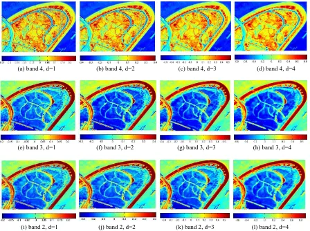
respectively. In experiments, we take different values for d, which do not make the window width (2d+1) exceed the maximum range of the typical object classes. By table 1, the maximum range is within 8~9 pixels, so the proper value for d is 1, 2, 3 and 4. For each spectral band, its spatial autocorrelation bands calculated by different parameter ds are visualized as images (figure 5).
Figure 5 show that for each spectral band of original image, typical object classes (vegetation, water and road) in their spatial autocorrelation images are visible, and by the color bar, red regions and blue regions in autocorrelation images represent higher and lower autocorrelation degree, which correspond to “hot spots” and “cold spots” in original image, respectively. The autocorrelation images include most structure information of the object classes and filter out some small detailed information.
(a) band 4, d=1 (b) band 4, d=2 (c) band 4, d=3 (d) band 4, d=4
(e) band 3, d=1 (f) band 3, d=2 (g) band 3, d=3 (h) band 3, d=4
(i) band 2, d=1 (j) band 2, d=2 (k) band 2, d=3 (l) band 2, d=4
Figure 5. Spatial autocorrelation images of different spectral bands with different window parameter ds
4.3 FCM clustering segmentation incorporating spatial
autocorrelation features
In this section, two segmentation experiments are conducted via the Fuzzy C-Means (FCM) algorithm, which employ the images of site 1 and site 2, respectively. The feature vectors for clustering segmentation consist of spectral features (three bands) and spatial autocorrelation features (also three bands). For comparison, the segmentation experiments only employing spectral features are also conducted.
In the first experiment, the image of site 1 is used for clustering
segmentation. As the experiment focuses on the segmentation of three typical object classes (vegetation, water and road), cluster number is set as C=4. When iterating 30 times, segmentation results are shown in figure 6 (a) and figure 7, where figure 6(a) is the result of FCM clustering only employing spectral features of three bands while figure 7 are the ones that employ both spectral features and spatial autocorrelation features (three spectral bands and their spatial autocorrelation bands).
The second experiment uses the image of site 2 and for the segmentation of five typical object classes, cluster number is set as C=6. When iterating 50 times, segmentation results of FCM clustering are shown in figure 6 (b) and figure 8, where figure 6
(b) is the result of FCM clustering only employing spectral features of three bands while figure 8 are the ones that employ
both spectral features and spatial autocorrelation features.
(a) site 1 (b) site 2
Figure 6. Results of FCM clustering segmentation only employing spectral features
(a) d=1 (b) d=2 (c) d=3 (d) d=4
Figure 7. Results of FCM clustering segmentation employing both spectral features and spatial autocorrelation features in site 1 when window width (2d +1) is less than the maximum range
(a) d=1 (b) d=3 (c) d=5 Figure 8. Results of FCM clustering segmentation employing both spectral features and spatial autocorrelation features in site 2
when window width (2d +1) is less than the maximum range
Due to spectral variability, the segmentation results in figure 6, which only employs spectral features in FCM algorithm, look “broken” and include too many noise-like speckles which reduce the homogeneity of segments.
However, FCM clustering segmentation incorporating spatial autocorrelation features can obtain more homogeneous segments or objects (figure 7 and figure 8). Since window parameter d has great effect on calculation of local spatial autocorrelation, it also affects the results of clustering segmentation. Figure 7 and figure 8 show that as d increases, noise-like speckles disappear gradually, and segments are becoming more and more homogeneous, but when window width (2d+1) approaches the maximum range of all the semivariograms characterizing the selected object classes, the edges of some small objects begin to become fuzzy and even disappear gradually.
These facts show that the Getis statistic plays the role of a low-pass filter and spatial autocorrelation features can effectively suppress noise caused by spectral variability in FCM clustering segmentation. Therefore, this method can improve the quality of FCM clustering segmentation and obtain more homogeneous objects. However, there's one point which needs
attention that improvement of segmentation quality does not necessarily mean the improvement of classification accuracy.
5. CONCLUSION
This paper focuses on the analysis and modelling of spatial autocorrelation features for improving the segmentation quality of high resolution satellite images. The semivariograms are used to model spatial variability of typical object classes while Getis statistic is used to calculate the degree of local spatial autocorrelation. Segmentation experiments are conducted via the Fuzzy C-Means (FCM) algorithm, which incorporate both spatial autocorrelation features and spectral features. The results show that spatial autocorrelation features play the role of a low-pass filter which can suppress noise caused by spectral variability and therefore improve the segmentation quality.
For future research, we will focus on the determination of optimal neighborhood window width within the range of the semivariograms by quantitative evaluation on segmentation quality or classification accuracy.
6. ACKNOWLEDGEMENT
This research has been partially supported by the National Key Basic Research and Development Program (2012CB719903), by National Natural Science Foundation of China (61172175) and by the Fundamental Research Funds for the Central Universities (201121302020010).
7. REFERENCES
Akcay, H. G. & Aksoy, S., 2008. Automatic detection of geospatial objects using multiple hierarchical segmentations. IEEE Transactions on Geoscience and Remote Sensing, 46(7), pp. 2097-2111.
Balaguer, A., Ruiz, L. A., Hermosilla, T. & Recio, J. A., 2010. Definition of a comprehensive set of texture semivariogram features and their evaluation for object-oriented image classification. Computers & Geosciences, 36(2), pp. 231-240.
Bezdek, J. C., 1981. Pattern Recognition with Fuzzy Objective Function Algorithms. Plenum, New York.
Byun, Y., Kim, D., Lee, J. & Kim, Y., 2011. A framework for the segmentation of high-resolution satellite imagery using modified seeded-region growing and region merging. International Journal of Remote Sensing, 32(16), pp.4589-4609.
Franklin, S. E., Wulder, M. A. & Lavigne, M. B., 1996. Automated derivation of geographic window sizes for use in remote sensing digital image texture analysis. Computers & Geosciences, 22(6), pp. 665-673.
Johnson, B. & Xie, Z., 2011. Unsupervised image segmentation evaluation and refinement using a multi-scale approach. ISPRS Journal of Photogrammetry & Remote Sensing, 66(4), pp.473-483.
Meer, F. V., 2012. Remote sensing image analysis and geostatistics. International Journal of Remote Sensing, 33(18), pp. 5644-5676.
Myint, S. W., Wentz, E. A. & Purkis, S. J., 2007. Employing spatial metrics in urban land-use/land-cover mapping: comparing the Getis and Geary indices. Photogrammetric Engineering & Remote Sensing, 73(12), pp. 1403-1415.
Ord, J. K. & Getis, A., 1995. Local spatial autocorrelation statistics: distributional issues and an application. Geographical Analysis, 27(4), pp. 286-306.
Wulder, M. & Boots, B., 1998. Local spatial autocorrelation characteristics of remotely sensed imagery assessed with the Getis statistic. International Journal of Remote Sensing, 19(11), pp. 2223-2231