SINGLE-IMAGE SUPER RESOLUTION FOR MULTISPECTRAL REMOTE SENSING
DATA USING CONVOLUTIONAL NEURAL NETWORKS
L. Liebel∗, M. K¨orner
Technical University of Munich, Remote Sensing Technology, Computer Vision Research Group, Arcisstraße 21, 80333 Munich, Germany –{lukas.liebel, marco.koerner}@tum.de
WG ICWG III/VII
KEY WORDS:Single-Image Super Resolution, Deep Learning, Convolutional Neural Networks, Sentinel-2
ABSTRACT:
In optical remote sensing, spatial resolution of images is crucial for numerous applications. Space-borne systems are most likely to be affected by a lack of spatial resolution, due to their natural disadvantage of a large distance between the sensor and the sensed object. Thus, methods forsingle-image super resolutionare desirable to exceed the limits of the sensor. Apart from assisting visual inspection of datasets, post-processing operations—e.g.,segmentation or feature extraction—can benefit from detailed and distinguishable structures. In this paper, we show that recently introduced state-of-the-art approaches for single-image super resolution of conventional photographs, making use ofdeep learningtechniques, such asconvolutional neural networks (CNN), can successfully be applied to remote sensing data. With a huge amount of training data available,end-to-end learningis reasonably easy to apply and can achieve results unattainable using conventional handcrafted algorithms.
We trained our CNN on a specifically designed, domain-specific dataset, in order to take into account the special characteristics of multispectral remote sensing data. This dataset consists of publicly available SENTINEL-2 images featuring 13 spectral bands, a ground resolution of up to10 m, and a high radiometric resolution and thus satisfying our requirements in terms of quality and quantity. In experiments, we obtained results superior compared to competing approaches trained on generic image sets, which failed to reasonably scale satellite images with a high radiometric resolution, as well as conventional interpolation methods.
1. INTRODUCTION
As resolution has always been a key factor for applications using image data, methods enhancing the spatial resolution of images and thus actively assist in achieving better results are of great value.
In contrast to classicalsuper resolutionapproaches, using multiple frames of a scene to enhance their spatial resolution,single-image super resolutionalgorithms have to solely rely on one given input image. Even though earth observation missions typically favor orbits allowing for acquisition of the same scene on a regular basis, the scenes still change too fast in comparison to the revisit time, e.g.,due to shadows, cloud or snow coverage, moving objects or, seasonal changes in vegetation. We hence tackle the problem, as if there was no additional data available.
Interpolation methods, like bicubic interpolation, are straight-forward approaches to solve the single-image super resolution problem. Recent developments in the field of machine learning, particularly computer vision, favorevidence-basedlearning tech-niques using parameters learned during training to enhance the results in the evaluation of unknown data. By performing end-to-endlearning with vast training datasets for optimizing those parameters,deep learningtechniques, most prominently convo-lutional neural networks (CNNs)are actually able to enhance the data in an information-theoretical sense. CNN-based single-image super resolution methods therefore are not bound to the same restrictions as common geometric interpolation methods exclu-sively working on the information gathered in a locally restricted neighborhood.
Applications include but are not restricted to tools aiding the visual inspection and thus try to improve the subjective quality
∗Corresponding author
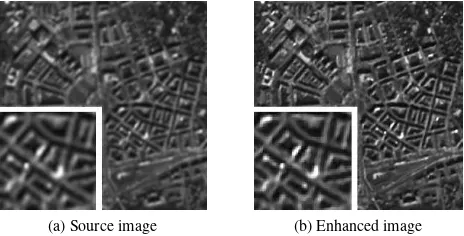
(a) Source image (b) Enhanced image
Figure 1: Enhancement of spatial resolution through single-image super resolution
as to be seen in Figure 1. Single-image super resolution methods can be efficiently used as pre-processing operations for further manual or automatic processing steps, such as classification or object extraction in general. As a wide range of remote sensing applications use such operations, the adaption of state-of-the-art single-image super resolution methods is eminently valuable.
experiments furthermore revealed system-inherent problems when applying deep-learning-based super resolution approaches to mul-tispectral satellite images and thus give indications on how to successfully adapt other related methods for remote sensing appli-cations as well.
The remainder of this paper is structured as follows: Section 2 introduces essential concepts and puts our work in the context of other existing approaches. In Section 3, starting from a detailed analysis of the problem, we present our methods, especially our ap-proach to address the identified problems. Extensive experiments to implement and prove our approach are described in Section 4. For this purpose, the generation of an appropriate dataset is shown in Section 4.2. The training process as well as results for a ba-sic and an advanced approach are presented in Section 4.3 and Section 4.4. Based on our experiments, we discuss the method and its results in Section 5 and compare them to other approaches followed by a concluding summary containing further thoughts on potential extensions in Section 6.
2. RELATED WORK
The term super resolution is commonly used for techniques using multiple frames of a scene to enhance their spatial resolution. There is however a broad variety of approaches to super resolution using single frames as their only input as well. Those can be divided into several branches, according to their respective general strategy.
As a first step towards super resolution, interpolation methods like the common bicubic interpolation and more sophisticated ones, like the Lanczos interpolation proposed by Duchon (1979), proved to be successful and therefore serve as a solid basis and reference for quantification.
Dictionary-based approaches, prominently based prominently on the work of Freeman et al. (2000) and Baker and Kanade (2000) focus on building dictionaries of matching pairs of high- and low-resolution patterns. Yang et al. (2008, 2010) extend these methods to be more efficient by using sparse coding approaches to find a more compact representation of the dictionaries. Recent work in this field, like (Timofte et al., 2013), further improve these approaches to achieve state-of-the-art performance in terms of quality and computation time.
Solving problems using deep learning has recently become a promising tendency in computer vision. A successful approach to single-image super resolution using deep learning has been pro-posed by Dong et al. (2014, 2016). They present a CNN, which they refer to asSRCNN, capable of scaling images with better results than competing state-of-the-art approaches.
CNNs were first proposed by LeCun et al. (1989), in the context of an application for handwritten digit recognition. LeCun et al. (1998) further improved their concept, but it only became a striking success when Krizhevsky et al. (2012) presented their exceptionally successful and efficient CNN for classification of the IMAGENETdataset (Deng et al., 2009). Especially the ability to train CNNs on GPUs and the introduction of therectified linear unit (ReLU)as an efficient and convenient activation function for deep neural networks (Glorot et al., 2011), enabled for work featuring deep CNNs as outlined by LeCun et al. (2015). Soft-ware implementations like the CAFFEframework (Jia et al., 2014) further simplify the process of designing and training CNNs.
The following section contains detailed information about the work of Dong et al. (2014, 2016) and the SRCNN.
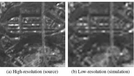
(a) High-resolution (source) (b) Low-resolution (simulation)
Figure 2: Low-resolution simulation
3. A CNN FOR MULTISPECTRAL SATELLITE IMAGE SUPER RESOLUTION
As shown in Section 2, there are promising CNN-based approaches available in the computer vision research field to tackle the single-image super resolution problem. In this section we examine prob-lems of utilizing a pretrained network to up-scale multispectral satellite images in Section 3.1 and further present our approach to overcome the identified problems in Section 3.2.
3.1 Problem
As motivated in Section 1, single-image super resolution methods focus on enhancing the spatial resolution of images with using one image as their only input.
Multispectral satellite images, as acquired by satellite missions like SENTINEL-2, differ significantly from photographs of objects recorded with standard hand-held cameras, henceforth referred to asconventional images. Particularly with regard to resolution, there is a big difference between those types of images.
Despite the rapid development of spaceborne sensors with amaz-ingly lowground sampling distance (GSD), and thus highspatial resolution, the spatial resolution of satellite images is still limited and very low in relation to the dimensions of the sensed objects. A 244×244 pxcut-out detail of a SENTINEL-2 image as prepared for our dataset (cf. Section 4.2) may cover the area of a whole town, while an equally sized image from the ImageNet dataset will typically depict a single isolated object in a much lower scale and therefore in superior detail.
This turns out to be a serious problem for deep learning approaches as training data consisting of pairs of matching low- and high-resolution images is needed in order to learn an optimal mapping. There is obviously no matching ground truth if the actual images are used as the low-resolution images to be up-scaled, since this would acquire images of even higher resolution. The only way to get matching pairs of training data therefore is to simulate a low-resolution version of the images. Looking ahead at the approach described in the following section, this is done through subsequently sampling the images down and up again.
10 m
20 m
60 m Visible
500 1000 1500 2000
Wavelength [nm]
Spati
al
R
esol
uti
on
Figure 3: SENTINEL-2 bands adapted from Sentinel-2 User Hand-book (2013)
be significantly harder to distinguish because of increasing blur. Figure 2 exemplary shows a cropped image of an urban scene with noticeable aliasing effects on the left side and heavily blurred areas especially observable on the right side, where former dis-tinct details become completely indistinguishable. Nevertheless, reconstruction might still be possible using evidence-based end-to-end learning methods, while the quality of results will be most certainly affected negatively. Since this issue applies to testing as well, results on the other hand might actually be even better than the quantification in Section 4 suggests, due to the lack of appropriate testing data.
Using a dataset as briefly described above will yield an optimal parameter set for the up-scaling of images from the simulated to the original spatial resolution. As this is certainly not the actual use case, we have to explicitly assume similar changes in low-level image structures while scaling from simulated low-resolution to the original resolution and from original resolution to the desired high-resolution.
Regardingspectral resolution, the large number of channels ac-quired simultaneously is a defining property of multispectral im-ages. SENTINEL-2 datasets, for instance, contain 13 channels, as shown in Figure 3 and characterized in detail in Section 4.2. Conventional images, in contrast, typically consist of exactly three channels (RGB), covering the visible spectrum exclusively.
Radiometric resolution, describing the number of discrete inten-sity values for each band, is a key difference between the images of the mentioned datasets. Unlike most standard camera sen-sors, acquiring images with a sampling depth of8 bit/px, sensors for multispectral remote sensing usually feature a much higher dynamical range. For instance, the sensors aboard the SENTINEL -2 satellites acquire images with a sampling depth of12 bit/px (Sentinel-2 User Handbook, 2013).
In our experiments (cf.Section 4), we analyzed the impact of the mentioned differences for a CNN trained on conventional images and evaluated for SENTINEL-2 singleband images.
3.2 Approach
The SRCNN is designed to perform single-image super resolution of monochrome8 bit/pxluminance channel images. They con-vert RGB images to YCbCr color space and apply SRCNN scaling to the Y-channel exclusively, while scaling the chrominance chan-nels by bicubic interpolation. Evaluated on common datasets containing conventional ImageNet-like images like SET5 used by Wang et al. (2004) and SET14 used by Zeyde et al. (2010), their approach achieved results superior to competing state-of-the-art methods.
Designed to work similar to autoencoders, extracting low-reso-lution patches and mapping them to high-resolow-reso-lution patches, the
Input
data label
Convolution 1
Kernel Size: 9 px
conv1 ReLU
Convolution 2
Kernel Size: 1 px
conv2 ReLU
Convolution 3
Kernel Size: 5 px
conv3
Loss
Type: Euclidean
loss 64
32
1
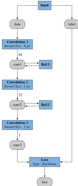
Figure 4: SRCNN Architecture
network topology as shown in Figure 4 consists of three inner layers. In addition to those intermediate layers, there are layers for data input and loss calculation.
Dong et al. (2014) analyze several networks with varying kernel sizes for the convolutional layers. We use the 9-1-5 version, as shown in Figure 4 and described later.
All of the inner layers are convolutional layers with a kernel size of9×9 pxin the first,1×1 pxin the second and5×5 px in the third layer. Apart from the layers, represented by blue rectangles, Figure 4 also shows the temporary storage elements used by Caffe, so-calledblobs, represented by grey octagons. The first convolution is applied to the “data” blob, populated by the input layer with a low-resolution version of the source image. As the network itself will not change the size of the input image, the input images are scaled to the desired output size using bicubic interpolation and a fixed scale.
A convolution with a kernel size of1 pxmight seem confusing at first, but considering the number of input and output channels, the filters learned are actually 3D filters with a dimensionality of 1×1×64. This is equivalent to a non-linear mapping between the low-resolution patterns extracted by the first convolution and the high-resolution patterns reconstructed by the third convolution in terms of the autoencoder analogy used by Dong et al. (2014).
The network can handle input image pairs,i.e.,source image and ground-truth images, of arbitrary size, as long as their dimensions match each other in the loss computing layer. Due to the bound-ary treatment of the network, the source image will be cropped by12 pxin width and height during a forward pass through the network. To compensate for this, the ground-truth image has to be smaller than the low-resolution source image.
The loss layer computes a loss value, quantifying the discrep-ancy or distance between the two input images. The precise loss function, calledEuclidean loss, evaluated by the loss layer in the SRCNN is
and provides a distance similar to themean squared error (MSE). HereNis the number of images in the currently processedmini batch,Dis the set of low-resolution “data” images andLis the set of high-resolution “label” images. The parameter vectorθ comprises filter weights and biases applied to the source images via the mapping functionF. During the training phase, a so called mini batch of training images is evaluated in parallel, where the number of images in a mini batch is much smaller than the number of images in the training set.
Dong et al. (2014) propose to train their network on either a small dataset with91images or a larger subset of the ImageNet with approximately400 000images. Since they showed that the training results of both datasets differ insignificantly, we used the smaller dataset in our experiments outlined in Section 4.
Given the results of Dong et al. (2014) and our own experiments in Section 4.3, we assume that it is generally possible to scale images using this network successfully. However, as shown in Section 3.1, multispectral satellite images differ from generic images in several critical properties. We assume scaling remote sensing images using the same technique is still possible, due to the fact that the differing properties only affect the parameters of the network, not the structure of the network itself. In end-to-end learning, the parameters in turn only depend-to-end on the provided training data. Thus, our approach on single-image super resolution for multispectral remote sensing data is training a CNN proven to have the desired capabilities with a suitable dataset. We describe the generation of such dataset in Section 4.2. With using a dataset, matching the test dataset in its properties considerably better, we are able to successfully apply the method to multispectral satellite imagery, as shown in Section 4.4.
4. EXPERIMENTS
In this section we describe our experiments conducted to verify our methods introduced in Section 3. The generation of the dataset we used for our experiments is described in Section 4.2. Section 4.3 and Section 4.4 feature detailed descriptions of the evaluation pro-cess and the corresponding results for both the basic and advanced method.
4.1 Quantification Metrics
In order to to quantify the results we mainly rely on thepeak signal-to-noise ratio (PSNR), commonly used for the evaluation of image restauration quality. Even though we use the PSNR for evaluation purposes, it is not used as a loss function for the optimization of any of the CNNs presented in this paper, mainly due to its higher computational effort. The euclidean loss, cf. Equation (1), minimized by the solver algorithm, however, is closely related to the MSE
dMSE= 1
which in turn favors a high PSNR
dPSNR= 10·log10
depending solely on the MSE andvmax = 2b
−1, a constant representing the upper bound of possible intensity values.
Beside the PSNR we evaluated thestructural similarity (SSIM) index (Wang et al., 2004) for our test dataset. This measure is designed to be consistent with human visual perception and, since scaling images for further manual processing is an important application for single-image super resolution, this metric seems to be well suited for our evaluation purposes.
4.2 Multispectral Dataset
The availability of suitable images for training in large quantities is a key requirement deep learning in general and our approach in particular. In this section we describe the, for the most part automatic, generation of a multispectral satellite image dataset for training and testing our network, more specifically the learned parameters.
The COPERNICUSprogramme funded by theEuropean Commis-sionprovides free access to the earth observation data of the dedi-cated SENTINELmissions and the contributing missions (Coper-nicus Sentinel Data, 2016). The SENTINEL-2 mission is mainly designed for land and sea monitoring through multispectral imag-ing. SENTINEL-2A, the first satellite out of two in the planned constellation was launched in June 2015, SENTINEL-2B is ex-pected to follow later in 2016. Each of the two carries or will carry a multispectral imaging sensor, the so called MULTISPECTRAL INSTRUMENT(MSI), acquiring images with a radiometric resolu-tion of12 bit/px. Figure 3 shows the bands acquired by the MSI, as well as their respective spatial resolution. All areas covered by the acquisition plan will be revisited at least every five days. For our dataset, we used Level-1C ortho-images containing top of atmosphere reflectances, encoded in16 bit/pxJPEG2000 format.
Our dataset is composed of75SENTINEL-2granules, covering an area of100 km2
Figure 5: Source image locations. Background map: c
OPENSTREETMAP contributors, available under the OPEN DATABASELICENSE
We sub-divided the images to244×244 pxtiles to simplify the data management and selection process. The resulting set of tiles contains images with no-data values, due to the discrepancy be-tween the area covered by the acquired images and the distributed granule grid, insignificant for the training process. The same holds true for tiles with little to no structure in their content or monotonous areas like large water bodies, grassland, and agricul-tural areas. To remove those unsuited tiles, we used statistical metrics,e.g.,shannon entropy with an absolute threshold and a check for no-data values. If a tile failed at least one of the tests, it was omitted from further processing. Out of the remaining set of tiles, we randomly chose a subset of 4096 tiles for training and 128 tiles for testing.
We generated a low-resolution simulation, as discussed in Sec-tion 3.1, of the datasets by subsequently sampling the images down and up again, according to the desired scale factor of2, using bicubic interpolation and clipping the results to a range of0 to216
−1.
At this stage of the process, we have got a multi-purpose dataset consisting of pairs of low- and high-resolution images with 13 channels. Training the CNN, however, requires pairs of normal-ized monochromatic patches in double- or single-precision, ac-cording to the capacities of the GPU available.
As converting multispectral images to YCbCr color space, as proposed by Dong et al. (2014), is neither possible nor desirable we approach the multichannel dataset as a set of singleband images. Without loss of generality, we picked the MSI B03 singleband images, representing the green channel of the dataset, for our experiments. Tiling once more yields33×33 pxlow-resolution data patches and21×21 pxhigh-resolution label patches with a stride of14 pxas proposed by Dong et al. (2014). The datasets are stored as normalized double-precision floats in several files formatted as HDF5 (The HDF Group, 1997-2016).
4.3 SRCNN
In order to test the results of the original SRCNN network and dataset combination for remote sensing data, we trained the net-work using the Caffe configuration files and Matlab functions for dataset creation provided along with (Dong et al., 2014). We used the 9-1-5 topology described in Section 3.2. The number of pa-rameters to be optimized in a network consisting of convolutional
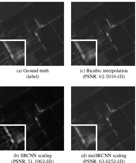
(a) Ground truth (label)
(b) SRCNN scaling (PSNR:51
.1962 dB)
(c) Bicubic interpolation (PSNR:62
.5918 dB)
(d) msiSRCNN scaling (PSNR:63
.6252 dB)
Figure 6: SENTINEL-2 B03 singleband image scaling
layers as inner layers exclusively can be derived by
|Θ|=
I X
i=1
ni·ci·hi·wi+ni, (4)
whereIis the number of convolutional layers,nis the number of filters,i.e.,output channels to be learned,cis the number of input channels, andh, ware the kernel height and width, respectively. As solely square filters are used in the networks evaluated in our experiments,h=wholds in all cases.
There are approximately8000parameters to be optimized in this version of the SRCNN. The optimization of the network param-eters was done using astochastic gradient descent (SGD)solver with a fixed learning rate ofη = 0.001and a fixed number of 1.5·107
iterations. Given a mini batch size of128patches, the optimization was performed through1.92·109
backpropagations. The training took approximately20 dayson a single NVIDIA TESLAK40C GPU.
Since Dong et al. (2014) already proved the SRCNN to success-fully scale8 bit/pxmonochrome luminance channel images, we proceeded to evaluate the learned parameter set with our test dataset. The quantitative and qualitative results are summarized in Table 1 and exemplary shown in Figure 6, respectively. Sec-tion 5 contains a discussion of the results in the context of further experiments as described in the following section.
4.4 msiSRCNN
Table 1: Scaling results for our test dataset
Network Measure Absolute (CNN) Difference (CNN−Bicubic)
mean max min mean max min
SRCNN PSNR [dB] 51.2227 52.3962 51.1588 −9.0618 −1.3529 −17.8358
SSIM 0.7673 0.9856 0.4812 −0.2304 −0.0113 −0.5178
msiSRCNN PSNR [dB] 60.6527 69.3490 52.9041 0.3682 1.0334 0.0725 SSIM 0.9979 0.9999 0.9536 0.0002 0.0068 0.0000
0 0
.5 1 1.5 2 2.5 3 3.5
·10
6 1.6
1.7 1.8 1.9·10
−3
Iterations (`a 256 Backpropagations)
T
esting
Loss
(Euclidean)
Figure 7: Change of loss
Aside the replacement of the dataset, we used an adjusted solver with a fixed learning rate ofη= 0.01and a mini batch size of256 patches. In our experiments, we observed faster convergence and a higher stability of loss for our optimized settings, as opposed to the original solver settings. The training was conducted on the same NVIDIA TESLAK40C GPU as before and took approximately 10days for3.5·106
iterations or8.96·108
backpropagations. Figure 7 shows the change of loss during the training process. The results for our set of test images are summarized in Table 1 and exemplary shown in Figure 6.
As mentioned before (cf.Section 1), the actual use case for super-resolution techniques usually differs from the experiments con-ducted, since quantification is impossible without a high resolution reference. The existence of a high-resolution version of the source image in turn supersedes the need to up-scale the image in the first place. Figure 8 shows an example of actual super-resolution using an input image in original resolution rather than a simulated low-resolution version, with the msiSRCNN scaling showing less overall blur compared to the bicubic interpolation.
Section 5 discusses the results in the context of more experiments as described in the previous section.
We conducted further experiments on scaling all of the channels of multispectral images. Table 2 and Figure 9 contain results for the RGB channels exclusively, since they can be interpreted easily.
5. DISCUSSION
We were able to reproduce the results obtained by Dong et al. (2014) for conventional luminance channel images. Table 1 and Figure 6, however, suggest that scaling SENTINEL-2 singleband images using the SRCNN yields unsatisfying results, as the net-work in fact impairs the quality of the input images, scaled to desired size using bicubic interpolation during pre-processing (cf.
(a) Bicubic interpolation
(b) msiSRCNN scaling
Figure 8: Actual up-scaling of a high-resolution input image
(a) Bicubic interpolation (PSNR:62
.6901 dB)
(b) msiSRCNN scaling (PSNR:63
.2563 dB)
(c) Ground truth (label)
Table 2: Scaling results for our test dataset in RGB
Channel Measure Absolute (msiSRCNN) Difference (msiSRCNN−Bicubic)
mean max min mean max min
B04 (Red) PSNR [dB] 58.8576 67.8606 52.5745 0.2191 1.4024 −1.7709
SSIM 0.9965 0.9998 0.9545 0.0002 0.0068 −0.0018
B03 (Green) PSNR [dB] 60.6527 69.3490 52.9041 0.3682 1.0334 0.0725 SSIM 0.9979 0.9999 0.9536 0.0002 0.0068 0.0000
B02 (Blue) PSNR [dB] 62.2797 68.7906 52.7989 0.3103 0.7500 0.0641 SSIM 0.9984 0.9998 0.9519 0.0002 0.0067 0.0000
RGB Composite PSNR [dB] 58.2760 68.5833 36.2356 −1.7475 0.5662 −16.3979
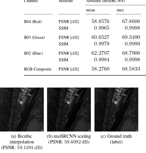
(a) Bicubic interpolation (PSNR:59
.1391 dB)
(b) msiSRCNN scaling (PSNR:59
.6092 dB)
(c) Ground truth (label)
Figure 10: msiSRCNN scaling results for a scene located outside the area covered by the training and testing datasets
Section 3. We therefore consider SRCNN scaling for multispectral satellite images as inadequate even though minor experiments con-ducted but not described in detail in this paper show that SRCNN scaling yields acceptable results for RGB composites of chan-nel satellite images, after extracting the luminance chanchan-nel and stretching their dynamic range to8 bit/px. The results still barely surpass bicubic interpolation. Further minor experiments imply problems when scaling images with a much higher dynamic range than the images used for training.
The optimization of a parameter set gained from re-training the SRCNN with our generated dataset was successful, as the loss function converges after a moderate number of training iterations, as to be seen in Figure 7. The resulting msiSRCNN turned out to be able to successfully scale SENTINEL-2 singleband images, as Table 1 and Figure 6 reveal.
The images used in our datasets were acquired from a very lim-ited number of locations, which raises the questions whether the msiSRCNN is able to successfully scale images acquired under different conditions,i.e.,generalization is still ensured. In Fig-ure 10 we present the results for the scaling of an image which is part of a SENTINEL-2 granule neither included in our training nor testing dataset. These results suggest that the dataset used for training is generic enough, although this is, as mentioned before, not our main goal in this work.
As to be seen in Table 2 and exemplary shown in Figure 9, scal-ing bands other than the one used for trainscal-ing yields significantly poorer results. The msiSRCNN outperforms bicubic interpolation slightly, but clearly using a network optimized for a single band to scale bands unknown to the network is of moderate success. A straightforward approach towards compensating this issue is opti-mizing a dedicated set of parameters per channel. Since training the network with an appropriate dataset, like the one we prepared in Section 4.2, without any necessary further changes to the net-work or the solver is just a matter of a few days of training, we are
confident that this is a proper solution to the problem of scaling datasets contain multiple bands. We are aware of the fact that this approach excludes a large portion of the information contained in multispectral datasets and address this in Section 6.
6. SUMMARY & OUTLOOK
In this paper we showed the steps necessary to successfully adapt a CNN-based single-image super resolution approach for multispec-tral satellite images. By generating a dataset out of freely available SENTINEL-2 images, we were able to re-train the SRCNN in or-der for it to work on multispectral satellite images with a high radiometric resolution. Our experiments demonstrated the ability of our trained CNN to successfully scale SENTINEL-2 singleband images.
As suggested in Section 5, scaling a multichannel image can safely be assumed to be possible with specialized sets of parameters for each channel. However, looking at multispectral images as a batch of unrelated singleband images is a very restricted view of the information contained in such datasets. With feeding multichannel images as a whole to the CNN, optimizing parameters for the scaling of a complete multispectral dataset at once, this side-information could be made accessible. Working on such 3D arrays is well within the scope of the Caffe implementation. In fact, this is only a minor modification to the network architecture, since only the input layer and the very last convolutional layer are affected. The inner layers operate on 3D array of activation images anyway, as explained in Section 3.2. The only parameter that needs to be modified regarding network architecture is the number of filters to be learned in the last convolutional layer. Changing the number of input channels in the first convolutional layer, as well as the number of output channels in the last convolutional layer from one to13(cf.Figure 4), will however heavily affect the overall number of parameters to be optimized. As per Equation (4), this increases the total number of parameters from approximately8·103
by one order of magnitude to approximately8·104
.
Au contraire, using the spectral information inherent in each pixel and utilize,e.g.,implicit information about the surface material, an extended msiSRCNN is assumed to be able to produce better results due to the cross-band information being available. In order to implement these modifications, some inherent problems need to be solved. The SENTINEL-2 datasets used in our experiments vary in spatial resolution in their singleband images, as to be seen in Figure 3. Caffe, however, is only able to handle blocks of same-sized input images. Therefore, approaches to this preprocessing steps, such as scaling the lower-resolution bands to the highest resolution appearing in the dataset using standard interpolation methods, need to be developed.
To ensure convergence during optimization, a bigger dataset should be used for training, even though our training dataset already out-ranks the dataset successfully used by Dong et al. (2014) in terms of quantity. Certainly, the dataset also has to be extended to a matching number of channels. Our dataset, presented in Sec-tion 4.2, includes all of the 13 spectral bands, thus only the fully parameterized automatic patch-preparation is affected.
Early stage experiments showed promising results even though some of the mentioned problems still need to be resolved.
ACKNOWLEDGEMENTS
We gratefully acknowledge the support of NVIDIA CORPORA -TIONwith the donation of the Tesla K40 GPU used for this re-search.
References
Baker, S. and Kanade, T., 2000. Hallucinating faces. In: Proceedings of the IEEE International Conference on Automatic Face and Gesture Recognition (FG), pp. 83–88.
Copernicus Sentinel Data, 2016. https://scihub.copernicus.eu/ dhus, last accessed May 10, 2016.
Deng, J., Dong, W., Socher, R., Li, L. J., Li, K. and Fei-Fei, L., 2009. Imagenet: A large-scale hierarchical image database. In: Proceedings of the IEEE Conference on Computer Vision and Pattern Recognition (CVPR), pp. 248–255.
Dong, C., Loy, C. C., He, K. and Tang, X., 2014. Learning a deep con-volutional network for image super-resolution. In: D. Fleet, T. Pajdla, B. Schiele and T. Tuytelaars (eds), Proceedings of the European Con-ference Computer Vision (ECCV), Springer International Publishing, Cham, pp. 184–199.
Dong, C., Loy, C. C., He, K. and Tang, X., 2016. Image super-resolution using deep convolutional networks. IEEE Transactions on Pattern Analysis and Machine Intelligence (TPAMI) 38(2), pp. 295–307.
Duchon, C. E., 1979. Lanczos filtering in one and two dimensions. Journal of Applied Meteorology 18(8), pp. 1016–1022.
Freeman, W. T., Pasztor, E. C. and Carmichael, O. T., 2000. Learning low-level vision. International Journal of Computer Vision 40(1), pp. 25–47.
Glorot, X., Bordes, A. and Bengio, Y., 2011. Deep sparse rectifier neural networks. In: International Conference on Artificial Intelligence and Statistics (AISTATS), pp. 315–323.
Jia, Y., Shelhamer, E., Donahue, J., Karayev, S., Long, J., Girshick, R., Guadarrama, S. and Darrell, T., 2014. Caffe: Convolutional architecture for fast feature embedding. arXiv preprint arXiv:1408.5093.
Krizhevsky, A., Sutskever, I. and Hinton, G. E., 2012. Imagenet clas-sification with deep convolutional neural networks. In: F. Pereira, C. J. C. Burges, L. Bottou and K. Q. Weinberger (eds), Advances in Neural Information Processing Systems 25, Curran Associates, Inc., pp. 1097–1105.
LeCun, Y., Bengio, Y. and Hinton, G., 2015. Deep learning. Nature 521(7553), pp. 436–444.
LeCun, Y., Boser, B., Denker, J. S., Henderson, D., Howard, R. E., Hub-bard, W. and Jackel, L. D., 1989. Backpropagation applied to handwrit-ten zip code recognition. Neural computation 1(4), pp. 541–551.
LeCun, Y., Bottou, L., Bengio, Y. and Haffner, P., 1998. Gradient-based learning applied to document recognition. Proceedings of the IEEE 86(11), pp. 2278–2324.
Sentinel-2 User Handbook, 2013. https://earth.esa.int/ documents/247904/685211/Sentinel-2_User_Handbook, last accessed May 10, 2016.
The HDF Group, 1997-2016. Hierarchical Data Format, version 5.http: //www.hdfgroup.org/HDF5/, last accessed May 10, 2016.
Timofte, R., Smet, V. D. and Gool, L. V., 2013. Anchored neighborhood regression for fast example-based super-resolution. In: Proceedings of the IEEE International Conference on Computer Vision (ICCV), pp. 1920–1927.
Wang, Z., Bovik, A. C., Sheikh, H. R. and Simoncelli, E. P., 2004. Image quality assessment: from error visibility to structural similarity. IEEE Transactions on Image Processing (IP) 13(4), pp. 600–612.
Yang, J., Wright, J., Huang, T. and Ma, Y., 2008. Image super-resolution as sparse representation of raw image patches. In: Proceedings of the IEEE Conference on Computer Vision and Pattern Recognition (CVPR), pp. 1–8.
Yang, J., Wright, J., Huang, T. S. and Ma, Y., 2010. Image super-resolution via sparse representation. IEEE Transactions on Image Processing (IP) 19(11), pp. 2861–2873.