www.elsevier.com/locate/econedurev
A comparison of alternative specifications of the college
attendance equation with an extension to two-stage
selectivity-correction models
Michael J. Hilmer
*Visitor, Department of Economics, 130 FOB Brigham Young University, Provo, UT 84602-2363, USA
Received 29 January 1999; accepted 21 October 1999
Abstract
This paper estimates a college attendance equation for a common set of students using three popular econometric specifications: the multinomial logit, the ordered probit, and the bivariate probit. The results suggest that while the multinomial logit is rejected as an appropriate specification, the estimated marginal effects generally are not statistically different across the three specifications. Extending the analysis to two-stage corrections for selection bias suggests that the biggest potential for cross-specification differences occur in the estimated significance of the second-stage coef-ficients and the predicted outcomes based on those estimates. This suggests that for such applications it is likely important to carefully consider the choice of specification of the first-stage attendance equation.2001 Elsevier Science Ltd. All rights reserved.
JEL classification:I29
1. Introduction
A primary focus of the economics of higher education literature has been the college attendance decision. Within the voluminous literature estimating the factors that affect the college attendance decision three promi-nent econometric specifications have been used: the multinomial logit (Ordovensky, 1995; Savoca, 1991), the ordered probit (Hilmer, 1998; Broomhall & Johnson, 1994), and the bivariate probit (Evans & Schwab, 1995; Ganderton, 1992). As it is entirely possible that estimates differ significantly across specifications, the choice of specification may greatly influence the conclusions that can be drawn from the results. Moreover, most studies appear to give little consideration to the alternative empirical models but rather make a seemingly ad-hoc decision of which model to use. Consequently, it is important to develop some idea whether and by how
* Tel.:+1 (801) 378-2037; fax:+1 (801) 378-2844.
0272-7757/01/$ - see front matter2001 Elsevier Science Ltd. All rights reserved. PII: S 0 2 7 2 - 7 7 5 7 ( 0 0 ) 0 0 0 2 4 - 8
much parameter estimates differ across the different specifications. Unfortunately, previous studies have esti-mated the college attendance decision for different data sets and thus it is difficult to directly compare and con-trast those results.
of Lee (1983) type two-stage corrections for self-tion bias, we extend the analysis to consider such selec-tivity correction models. The estimated results for the years of college completed by 2- and 4-year attendees suggest that the choice of specification of the first-stage college attendance equation may have a significant impact on the second-stage selectivity-corrected coef-ficient estimates. Namely, the effects of several key vari-ables are estimated to be statistically significant under some specifications but not others. Prominent among these are test scores, which are only estimated to have large and significant effects among 4-year attendees for the ordered probit and a series of family background and high school performance measures, which are only esti-mated to have large and significant effects among 2-year attendees for the multinomial logit. In addition to the estimated coefficients differing across specifications, pre-dicted outcomes for students of different genders and ethnicities possessing average sample characteristics appear to differ across specifications. Hence, the results suggest the importance of considering specification issues before estimating the college attendance equation, especially when being used as the first stage of selection correction models.
2. Econometric issues
The econometric specifications examined in this study are well known and are all examples of discrete choice models.1In the context of college attendance, the models
all assume that a student makes his or her attendance decision on the basis of a latent variable, either the expected utility of an attendance option, the probability of college graduation, or more generally the underlying propensity to attend college. Unfortunately, the researcher does not directly observe the latent variable. Instead, he or she only observes the student’s actual attendance decision (for purposes of this study 4-year college attendance [Ei=2], 2-year college attendance
[Ei=1], or non-attendance [Ei=0]).2The discrete choice
models discussed below are all methods of
“back-1 Descriptions of the models analyzed in this study are available in most econometric texts. For a nice intuitive dis-cussion of these types of models see Kennedy (1998). For a more rigorous treatment, the classic references are Maddala (1983) and Greene (1997).
2 There may be some question as to the definition of 2-year colleges. In this study, a student is defined as attending a 2-year college if they are taking academic courses at a 2-2-year college. Students taking only vocational courses are defined as being non-attendees. All three models in this study could also have been estimated with vocational school defined as a separ-ate attendance path. As with Weiler (1989), doing so does not significantly alter the results.
tracking” from the observed attendance decision to the underlying relationships between certain explanatory variables and the attendance path decision. While the basic goals of the three models are the same, they differ according to the assumptions made about the relationship between the different attendance options.
2.1. Mutinomial logit
Estimation of the multinomial logit follows directly from expected utility maximization. As with other ran-dom utility models, the multinomial logit assumes that a student chooses which attendance path to follow by comparing the indirect utility provided by each path and choosing the one that provides the highest. For the cur-rent application, the student’s attendance path choice can be defined as:
where Xi is a vector of observed individual
character-istics and state-level relative net attendance costs that affect the student’s expect utility from each attendance option and ei is an i.i.d log Weibull distributed error
term.3 Parameters to be estimated by maximum
likeli-hood areB0,B1, andB2.
The multinomial logit has gained favor in estimating discrete choice models due to it computational ease. Namely, the probability of choosing each potential out-come can be easily expressed and the resulting log-likeli-hood function can be maximized in a straightforward fashion. A potential shortcoming of the multinomial logit is its reliance on the independence of irrelevant alterna-tives (IIA). The IIA property assumes that the relative probability of two existing outcomes is unaffected by the addition of a third outcome. For example, suppose that an individual’s choice is initially between two different outcomes and that he or she is evenly split between the two. Now, suppose we add a third alternative that is nearly identical to the second. We would then expect the probability of choosing the second outcome to be split in half and the probability of choosing the first outcome to be unaffected. Unfortunately, the IIA property does not account for this, but rather splits the probabilities equally among all three alternatives in order to keep the
relative probabilities of the first two options equal.4
Hence, in cases where two alternatives are close substi-tutes the multinomial logit may be inappropriate as it relies on the IIA property. Hausman and McFadden (1984) suggest a specification test, based on dropping a category from the estimation and observing whether the estimated coefficients change, that can be used to assess the validity of the IIA property in the model logit model. This test provides a means test whether the multinomial logit is an appropriate specification for this exercise.
2.2. Ordered probit
The ordered probit assumes that the variable of inter-est follows a strict ordering based on the value of the latent variable. Hilmer (1998) suggests that the latent variable is the student’s subjective probability of gradu-ation and that his or her decision follows the natural ordering of students with the highest probabilities attending 4-year colleges, students with midrange prob-abilities attending 2-year colleges, and students with the lowest probabilities attending neither institution.5
Accordingly, the student’s attendance path can be defined as:
where Xi is a vector of factor’s affecting the student’s
subjective probability of graduation andmiis a normally
distributed error term. a1 anda2partition the student’s
attendance path choice into the decision to attend a 4-year college, attend a 2-4-year college, or attend no post-secondary institution and therefore represent the mini-mum probability levels at which a student chooses to
4 As a simplified example, suppose that in the absence of 2-year colleges a student is equally likely to choose to attend a 4-year college (1/2) as to not attend college (1/2). Now, suppose the student is given the choice between a 2-year college and a 4-year college and assume that he or she views the two as perfect substitutes. We would then expect the probabilities of non-attendance, 2-year non-attendance, and 4-year attendance to be, 1/2, 1/4, 1/4. This is not how the multinomial logit treats the prob-abilities, however. Due to the IIA property, the multinomial logit treats the probabilities as 1/3, 1/3, 1/3 in order to keep the relative probabilities of non- and 4-year attendance constant.
5 Hilmer (1998) explains the intuition as follows: “To avoid the time cost associated with transferring, a student who thinks he or she is likely to graduate will start at a university. A student who is uncertain about his or her ability will start at a com-munity college since the foregone cost of the first 2 years will be much lower should he or she be forced to drop out. A student who is not likely to graduate will choose to work since doing so will make him or her better off than attending a community college for 2 years and dropping out.”
attend a 4-year college and a 2-year college. Parameters to be estimated by maximum likelihood ared,a1, anda2.
A primary difference between the multinomial logit and the ordered probit is that due to the assumed natural ordering the latter does not require the IIA property. However, for the model to be appropriate, the assumed natural ordering must be realistic. For example, the natu-ral ordering of 4-year/2-year/non-attendance seems reasonable (at least for students expecting to receive a Bachelor’s degree) due to the lower attendance cost at 2-year colleges and the transfer cost associated with transferring from a 2-year college to a 4-year college.6
On the other hand, if one were examining the decision between public and private 4-year colleges assuming a natural ordering of private/public may not be reasonable as it has been demonstrated that many students choose to attend public institutions that are potentially lower in quality than the private colleges they would have chosen in order to take advantage of the in-kind subsidy afforded by public higher education (Ganderton, 1992). This observation suggests that the estimated thresholds in the ordered probit model should always be significant. If not, then we might conclude that the assumed natural ordering and consequently the ordered probit is an inap-propriate specification for this exercise. While this obser-vation is potentially valuable in determining whether the ordered probit is inappropriate it would be of limited value in assessing whether it is superior to the alterna-tives models we are discussing.
2.3. Bivariate probit with sample selection
The bivariate probit with sample selection (Greene, 1998) assumes that the potential student makes two sequential decisions: (1) whether to attend a postsecond-ary institution and (2) if so which type of institution to attend. The model can thus be defined as:7
Z1i=f19X1i+e1i E2=1 ifZ1i.0 E1=1 otherwise
Z2i=f29X2i+e2i Z1iobservedif Z2i.0 E0=1 otherwise
(e1i,e2i)BVN(0,0,1,1,r)
(3)
6 Community college transfer students may be forced to take longer to graduate for a variety of reasons. For example, com-munity college students often take smaller class loads than uni-versity students, and as a result, are required to either spend longer taking classes at the community college before transfer-ring or at the university after transfertransfer-ring. Either way, such stu-dents will be required to spend longer in school before receiving their degree.
whereZ1iandZ2iare the latent variables determining the
attendance/non-attendance and 2-year/4-year attendance decisions,X1iandX2iare vectors of individual- and
state-specific characteristics affecting those decisions, and the error terms e1i and e2i are distributed bivariate normal
(BVN) with r representing the correlation coefficient between the two. Parameters to be estimated by maximum likelihood aref1,f2, andr.
As with the ordered probit, a potential benefit of the bivariate probit with sample selection is that by assuming the two attendance decisions are made sequentially, the model does not rely on the IIA property. A potential drawback is the requirement that the error terms from the two equations be distributed jointly normal. Due to this requirement, it should be possible to determine whether the model is inappropriate by testing whether the assumed joint normality of the two error terms holds. Again, while such a test is valuable in determining whether the bivariate probit with sample selection is inappropriate it would be of limited value in assessing whether a model for which joint normality is not rejected is superior to the models discussed above.
2.4. Correcting for self-selection bias
An application of the college attendance equation that has recently become popular is as the first-stage in two-stage econometric models that correct OLS estimates for the presence of self-selection bias. For example, Brewer, Eide and Ehrenberg (1999) estimate a multinomial logit selection model to correct for potential selectivity bias in the return to elite private colleges while Ganderton (1992) estimates a bivariate probit selection model to correct for potential selection bias in student quality choices at public and private universities. The problem inherent in such studies is that the observed outcomes are the result of non-random decisions. Namely, the return to quality for students attending elite, private institutions and the quality choices of students attending public and private universities are only observed for students mak-ing the non-random decisions to attend an elite, private institutions and public or private universities and not for the entire population of college-age students. As Heck-man (1979) and others demonstrate, this non-ran-domness, or self-selection of college attendance choices violates the familiar Gauss–Markov assumptions. Conse-quently, estimating the desired outcomes by OLS yields potentially biased results.
To correct for the potential of self-selection bias, most studies employ the two-stage methodology of Lee (1983). According to this methodology, it is possible to correct for the non-random assignment to different attendance paths by: (1) estimating the student’s self-selected college attendance choice and (2) using those results to calculate selectivity-correction terms that when included as regressors in the second-stage functions
cor-rect for the potential self-selection bias. The intuition behind this procedure is that the selectivity-correction terms are derived from the attendance path estimates and therefore include the important effect that a student’s unobservable characteristics have on his or her attend-ance path decision. Including those terms in the second-stage functions then corrects for the bias that may be induced by students with identical observable character-istics non-randomly self-selecting different attendance paths and subsequently making persistence decisions that differ due strictly to differences in their unobservable characteristics.
In the work below, we examine the effect that choice of specification for the college attendance equation has on the two-stage selectivity-corrected results by estimat-ing the years of college that a student completes. The econometric model to be estimated is a system of reduced form equations that can be specified as:
Eiestimated as a multinomial logit, ordered probit, (4)
or bivariate probit
Yi5h1Wi1h2li1ni (5)
where Yirepresents the number of years of college that
the student completes,Wiis a vector of observed
individ-ual characteristics affecting the student’s college persist-ence decision, li is the selectivity-correction term
derived from the first-stage Eq. (4), andniis a stochastic
error term. Parameters to be estimated areWiandli, with
Wirepresenting the selectivity-corrected results.
3. Data
Data for this analysis are drawn from the High School and Beyond (HSB) survey. The HSB is a US Department of Education longitudinal survey of a nationwide sample of students who were attending high school in 1980. The survey consists of two cohorts of students: roughly 12,000 high school seniors and roughly 15,000 high school sophomores (National Center for Education Stat-istics, 1987). Students were initially questioned in 1980 with follow-up surveys conducted in 1982, 1984, 1986, and 1992 (sophomores only). The survey is ideal for this study as it collects extensive information on students’ college attendance and early career work experiences.
sufficient information to calculate the variables of inter-est.
Several factors may influence a student’s college attendance decision. When making his or her initial attendance decision,8 the rational high school graduate
utilizes all available information to assess his of her expected utility of each attendance option. Presumably, several observable values affect this assessment. Individ-ual characteristics that affect a student’s graduation prob-ability are binary dummy variables indicating the stud-ent’s gender and ethnicity. Family background is measured by a categorical variable indicating the income of the student’s family in 19809 and a binary dummy
variable indicating whether at least one parent completed college. Measured academic ability is defined as the stu-dent’s average performance on math and reading tests administered during the senior year in high school. Vari-ables measuring high school experiences are a dummy variable indicating whether the student pursued an academic/college preparatory high school program, a categorical variable indicating the student’s self-reported high school grades, and a continuous variable rep-resenting the number of extracurricular activities in which the student participated during his or her senior year. Higher education expectations are measured by a binary dummy variable indicating whether the student reported that he or she expected to one day receive an advanced degree. Finally, a dummy variable indicating whether the student was initially questioned as a senior or a sophomore is included to control for potential sys-tematic differences between the cohorts.
The student’s initial attendance decision will also depend in large part on both the direct attendance and opportunity costs associated with each option. Direct attendance costs take the form of both tuition and fees and relative access to different types of institutions (which may force the student to move from home or face a longer commute). Opportunity costs take the form of foregone earnings during the period of attendance. Direct attendance costs are measured by the average tuition at and 4-year colleges and the ratio of the number of 2-and 4-year colleges to the number of students in the stud-ent’s home state (Office of Educational Research and
8 We use the term “initial” to represent the initial type of institution that a student attended rather than applying the term to a distinct time period. Most students who attended college did so in the first semester after high school graduation. How-ever, a minority of students waited until some later date and for them our definition of the initial decision reflects the first school they attended.
9 In the HSB survey, family income is a categorical variable. In $1980 the income categories are: (1),$7000; (2) $7000– $11,999; (3) $12,000–$15,999; (4) $16,000–$19,999; (5) $20,000–$24,999; (6) $25,000–$37,999; (7) $38,000 or more.
Improvement, 1997).10 Opportunity cost measures are
the 1982 unemployment rate and 1982 median wage in the student’s county of residence.
Finally, it is possible that there are state-specific dif-ferences in the propensity to attend college that may not be captured by differences in attendance costs. To account for such potential differences, we would like to include state-specific dummy variables. However, because attendance costs are entered on the state-level, we cannot include state dummies. Instead, we include an exhaustive set of dummy variables indicating the census region of the student’s high school (Pacific region excluded) to account for potential cross-region differ-ences in the propensity to attend college.
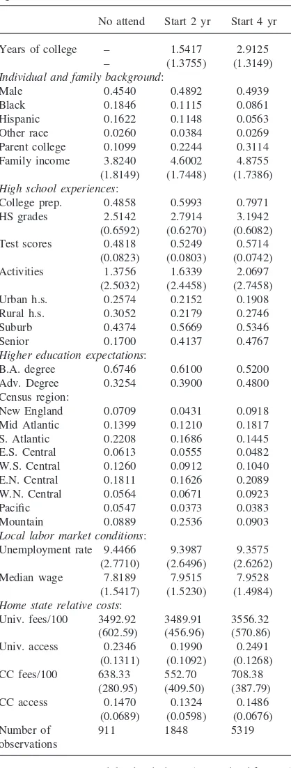
Table 1 presents summary statistics for the inde-pendent variables described above. Within this sample of HSB students who as high school seniors expected to graduate from college, 769 chose not to attend any col-lege, 1792 chose to enroll in a 2-year colcol-lege, and 5089 chose to enroll in a 4-year college. Comparing across the three attendance groups, students expecting to graduate from college who initially attend 4-year colleges com-plete nearly three full years of college while those who initially attend 2-year colleges complete roughly one and one-half years less. This difference is expected and is consistent with the finding in Rouse (1995) that HSB students who attend 2-year colleges might be “diverted” to complete fewer years of college than those who attend 4-year colleges.11Turning to independent variables,
non-attendees are most likely to be female, Black, and His-panic while 2-year attendees are more likely than 4-year
10 A well-known property of the HSB data set is that it does not include identifiers of the student’s home state. Most pre-vious studies have imputed home states following the back-tracking technique described in Ganderton (1992). According to that technique, the state in which most students from a high school attend college is likely the home state of the schools students. Using that procedure, it possible to unambiguously identify the home states of roughly 90% of all students. This study makes use of an alternative method for identifying home states. The HSB file contains the 1980 unemployment rate in each student’s home state. For 1980, there was enough variation in unemployment rates across census regions that it is possible to unambiguously identify each state. As a consequence, our data set contains a fuller sample as we do not have to exclude any students for missing state data. tive method for identifying home states. The HSB file contains the 1980 unemployment rate in each student’s home state. For 1980, there was enough variation in unemployment rates across census regions that it is possible to unambiguously identify each state. As a conse-quence, our data set contains a fuller sample as we do not have to exclude any students for missing state data.
Table 1
Summary statistics for students expecting to graduate from col-legea
No attend Start 2 yr Start 4 yr
Years of college – 1.5417 2.9125
– (1.3755) (1.3149)
Individual and family background:
Male 0.4540 0.4892 0.4939
Black 0.1846 0.1115 0.0861
Hispanic 0.1622 0.1148 0.0563
Other race 0.0260 0.0384 0.0269
Parent college 0.1099 0.2244 0.3114 Family income 3.8240 4.6002 4.8755 (1.8149) (1.7448) (1.7386) High school experiences:
College prep. 0.4858 0.5993 0.7971
HS grades 2.5142 2.7914 3.1942
(0.6592) (0.6270) (0.6082) Test scores 0.4818 0.5249 0.5714
(0.0823) (0.0803) (0.0742)
Activities 1.3756 1.6339 2.0697
(2.5032) (2.4458) (2.7458)
Urban h.s. 0.2574 0.2152 0.1908
Rural h.s. 0.3052 0.2179 0.2746
Suburb 0.4374 0.5669 0.5346
Senior 0.1700 0.4137 0.4767
Higher education expectations:
B.A. degree 0.6746 0.6100 0.5200 Adv. Degree 0.3254 0.3900 0.4800 Census region:
New England 0.0709 0.0431 0.0918 Mid Atlantic 0.1399 0.1210 0.1817 S. Atlantic 0.2208 0.1686 0.1445 E.S. Central 0.0613 0.0555 0.0482 W.S. Central 0.1260 0.0912 0.1040 E.N. Central 0.1811 0.1626 0.2089 W.N. Central 0.0564 0.0671 0.0923
Pacific 0.0547 0.0373 0.0383
Mountain 0.0889 0.2536 0.0903
Local labor market conditions:
Unemployment rate 9.4466 9.3987 9.3575 (2.7710) (2.6496) (2.6262) Median wage 7.8189 7.9515 7.9528
(1.5417) (1.5230) (1.4984) Home state relative costs:
Univ. fees/100 3492.92 3489.91 3556.32 (602.59) (456.96) (570.86) Univ. access 0.2346 0.1990 0.2491
(0.1311) (0.1092) (0.1268) CC fees/100 638.33 552.70 708.38
(280.95) (409.50) (387.79)
CC access 0.1470 0.1324 0.1486
(0.0689) (0.0598) (0.0676)
Number of 911 1848 5319
observations
a Notes: Data are weighted. Missing values omitted from cal-culations of seome means. Standard deviations in parentheses.
attendees to belong to those gender and ethnic groups. As with Hilmer (1998) and Ganderton (1992) family background appears to be important in the attendance decisions of HSB students. Students from families with higher incomes and with at least one parent who gradu-ated from college are more likely to attend a postsecond-ary institution and are most likely to attend a 4-year col-lege. Likewise, students who expect to receive advance degrees are most likely to attend 4-year colleges while those who expect only a Bachelor’s degree are most likely to choose not to attend any college.
Turning to the opportunity cost measures, students who attend no college come from counties with the high-est average unemployment rates while students who attend 2- or 4-year colleges come from counties with the highest average median wage rates, or highest expected returns to college attendance. At the same time, 2-year attendees live in states with the lowest average 2-year college fees and the highest relative 2-year college access, while 4-year attendees live in states with the highest average 2-year fees and lowest relative 2-year access.
4. Results
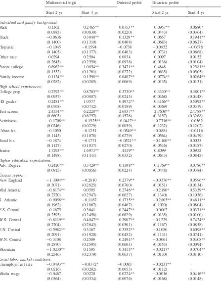
Table 2 presents the coefficient estimates for each of the three models by maximum likelihood.12These results
allow us to conduct some simple specification tests of the three models. The Hausman specification test for the multinomial logit strongly rejects the null hypothesis of IIA.13Hence, we can conclude that the multinomial logit
is not an appropriate specification for the attendance decision analyzed in this exercise. This is not at all sur-prising given that for students expecting to graduate from college, 2- and 4-year colleges may be reasonably close substitutes as they both allow the student a chance to
12 Maximum likelihood estimation of the multinomial logit model is straightforward. There are, however, two main practi-cal concerns in estimating the ordered probit and the bivariate probit models. First, for the ordered probit model to be ident-ified, we must make the assumption that in the likelihood func-tions2
i=1 (Greene, 1997, pp. 927–931). Second, for the bivari-ate probit model to be identified, the vectors of independent variables cannot be the same in both equations. Accordingly, we need to make an economically justifiable exclusion of some factor that influences the attendance/non-attendance decision but not the 2-year/4-year attendance decision. As preliminary analysis suggests that the county-level unemployment rate affects the attendance/non-attendance decision but not the 2-year/4-year attendance decision, we identify the model by excluding that variable form the latter estimation.
Table 2
Estimated coefficients for the three modelsa
Multinomial logit Ordered probit Bivariate probit
Start 2 yr Start 4 yr Start 2 yr Start 4 yr
Individual and family background:
Male 0.1362 0.2465** 0.0753** 0.0957** 0.0680*
(0.0883) (0.0830) (0.0220) (0.0443) (0.0364)
Black 20.0636 0.3048** 0.1329** 0.0657 0.1941**
(0.1400) (0.1310) (0.0408) (0.0683) (0.0627)
Hispanic 20.1045 20.1594 20.0738 20.0852 20.0678
(0.1405) (0.1377) (0.0463) (0.0731) (0.0668)
Other race 0.0294 0.2504 0.0834 0.0097 0.0132
(0.2645) (0.2550) (0.0938) (0.0136) (0.0104)
Parent college 0.6962** 1.0854** 0.3471** 0.4848 0.2581**
(0.1332) (0.1261) (0.0272) (0.0635) (0.0505)
Family income 0.1124** 0.1598** 0.0487** 0.0774** 0.0264**
(0.0282) (0.0265) (0.0069) (0.0135) (0.0131)
High school experiences:
College prep 0.2792** 0.8703** 0.3730** 0.3330** 0.3801**
(0.0937) (0.0887) (0.0243) (0.0468) (0.0448)
HS grades 0.2481** 1.0577 0.4972** 0.4166** 0.5092**
(0.0768) (0.0742) (0.0189) (0.0369) (0.0379)
Test scores 2.4554** 6.2228** 2.6837** 2.7608** 2.4788**
(0.6603) (0.6257) (0.1578) (0.3157) (0.3268)
Activitiess 20.1708** 20.1525** 20.0417** 20.7716** 20.0562
(0.0246) (0.0229) (0.0059) (0.1232) (0.1202)
Urban h.s. 20.1050 20.1251 20.0549** 20.0881 20.0116
(0.1143) (0.1078) (0.0279) (0.0564) (0.0479)
Rural h.s. 20.1874 20.1771 20.0521** 20.1160** 0.0035
(0.1127) (0.1037) (0.0270) (0.0546) (0.0487)
Senior 1.7293** 1.6974** .4119** 0.8099 0.0952
(0.1498) (0.1441) (0.0332) (0.0643) (0.0845)
Higher education expectations:
Adv. Degree 0.2420** 0.3429** 0.1198** 0.1769** 0.0786**
(0.0915) (0.0856) (0.0224) (0.0448) (0.0384)
Census region:
New England 21.3094** 20.2810 0.2379** 20.0376** 0.0596**
(0.3071) (0.2825) (0.0760) (0.0151) (0.0134)
Mid Atlantic 20.8174** 0.0595 0.2746** 20.2190* 0.5359**
(0.2720) (0.2547) (0.0627) (0.1340) (0.1036)
S. Atlantic 20.9058** 20.1167 0.1735** 20.2805** 0.4611**
(0.1962) (0.1867) (0.0467) (0.1020) (0.0804)
E.S. Central 20.1675 0.3641 0.2447** 20.0002 0.0371**
(0.2593) (0.2458) (0.0629) (0.0135) (0.0100)
W.S. Central 20.8119** 0.4047** 0.3907** 20.1229 0.7424**
(0.2204) (0.2043) (0.0501) (0.1167) (0.0858)
E.N. Central 20.5982** 0.3167 0.3352** 20.1080 0.6098**
(0.2091) (0.1920) (0.0452) (0.1131) (0.0741)
W.N. Central 20.3108 0.2509 0.2494** 20.0061 0.0408**
(0.2870) (0.2595) (0.0604) (0.0153) (0.0094)
Mountain 21.0230** 0.1595 0.3415** 20.0217* 0.0704**
(0.2546) (0.2379) (0.0637) (0.0130) (0.0110)
Local labor market conditions:
Unemployment rate 20.0493** 20.0372* 20.0083 20.0231** –
(0.0216) (0.0202) (0.0053) (0.0112) –
Media wage 20.0467 0.0220 0.0224** 20.0016 0.0416**
(0.0364) (0.0334) (0.0076) (0.0168) (0.0148)
Table 2 (continued)
Multinomial logit Ordered probit Bivariate probit
Start 2 yr Start 4 yr Start 2 yr Start 4 yr
Home state relative costs:
Univ. fees/100 0.0439** 0.0178 20.0009 0.0135 20.0088
(0.0190) (0.0169) (0.0042) (0.0098) (0.0071)
Univ. access 21.5235* 1.4231** 0.9215** 0.1851 1.5670**
(0.8195) (0.7260) (0.1772) (0.4199) (0.2854)
CC fees/100 20.0458* 0.0012 0.0100** 20.0005 0.0016**
(0.0250) (0.0194) (0.0036) (0.0015) (0.0005)
CC access 0.3917 0.0872 20.0309 20.0532 0.1310
(1.0620) (0.9555) (0.2519) (0.5348) (0.4550)
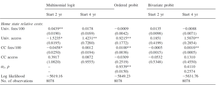
a2,r – 0.9339** 0.4110
– (0.0150) 0.2574
Log likelihood 25619.16 25849.23 25631.76
No. of observations 8078 8078 8078
a Notes: Estimation also includes dummy variables that are equal to one if values for a variable are missing (in which case those variables are set to zero). Data are weighted. Standard errors in parentheses. *, **Significant at the 5 and 10% levels.
pursue their goal while non-attendance does not. There-fore, we would expect that omitting one of those options (say 2-year attendance) would alter the relative prob-ability of the remaining two options (making 4-year attendance much more likely) thereby violating the IIA principle. Turning to the bivariate probit results, a likeli-hood ratio test rejects the null hypothesis that r=0 at the 1% level.14This provides evidence in favor of joint
normality between the error terms from the initial college attendance and the subsequent college type decisions, thereby suggesting that the bivariate probit with sample selection may be an appropriate specification for the attendance decision modeled in this exercise. Finally, for the ordered probit, the estimated threshold (between 2-and 4-year attendance as the threshold between non- 2-and 2-year attendance is scaled to 0) is highly significant which might suggest that the implied natural ordering is reasonable. Hence, based on our simple specification tests, we conclude that neither the ordered probit or the bivariate probit with sample selection can be statistically rejected as the correct econometric specifications.
It is well known that the coefficient estimates in Table
14 For the exercise, the restricted model is the one for which r=0, or for which probit equations are estimated separately for the two decisions. The unrestricted model is the one for which rÞ0 and the bivariate probit is estimated. The log-likelihood values for the separate probit equations are 22290.1962 and 23375.6948, respectively while the log-likelihood for the bivariate probit is 25631.76. Hence, the likelihood ratio test statistic is c2=22[(22290.1962+23375.6948) 2(25631.76)]=68.26. The 99% table value for a chi-square with one degree of freedom is 6.63. Therefore, we reject the null hypothesis thatr=0.
2 do not represent the true marginal effects of the inde-pendent variables and are therefore difficult to interpret (Greene, 1997, p. 916). The multinomial logit coef-ficients represent the effect that the independent vari-ables have on the probability of choosing 2- or 4-year attendance relative to the base category of non-attend-ance. The ordered probit coefficients represent the effect that the independent variables have on the likelihood of choosing one attendance path versus the other attendance paths. For example, suppose that high levels of family income are associated with 4-year college attendance. The ordered probit coefficient on FAMILY INCOME will then be positive and large in magnitude. Finally, the bivariate probit coefficients represent the effect that the independent variables have on the decision to attend either a 2- or 4-year college rather than no postsecondary institution and the decision of college attendees to attend a 2-year college rather than a 4-year college, respect-ively.
Table 3
Estimated marginal effects of selected characteristics on college attendancea
Multinomial logit Ordered probit Bivariate probit
No attend Start 2 yr Start 4 yr No attend Start 2 yr Start 4 yr Attend Start 4 yr
Individual and family background:
Male 20.0141 20.0147 0.0288** 20.0106 20.0158 0.0264 20.0032 0.0203
(0.0052) (0.0099) (0.0112)
Black 20.0142 20.0563** 0.0705** 20.0188 20.0278 0.0466 20.0022 0.0579
(0.0080) (0.0178) (0.0198)
Hispanic 0.0094 0.0068 20.0162 0.0104 0.0155 20.0259 0.0029 20.0202
(0.0083) (0.0179) (0.0206)
Other race 20.0128 20.0328 0.0457 20.0118 20.0175 0.0292 20.0003 0.0039
(0.0158) (0.0274) (0.0316)
Parent college 20.0636** 20.0487** 0.1122** 20.0490 20.0727 0.1218 20.0164 0.0770 (0.0095) (0.0123) (0.0140)
Family income 20.0095** 20.0055* 0.0150** 20.0069 20.0102 0.0171 20.0026 0.0079
(0.0018) (0.0032) (0.0036) High school experiences:
College prep. 20.0470** 20.0850** 0.1320** 20.0527 20.0782 0.1309 20.0113 0.1134
(0.0063) (0.0116) (0.0131)
HS grades 20.0558** 20.1183** 0.1741** 20.0702 20.1042 0.1744 20.0141 0.1520 (0.0061) (0.0103) (0.0110)
Test scores 20.3427** 20.5321** 0.8748** 20.3791 20.5624 0.9415 20.0935 0.7397
(0.0458) (0.0797) (0.0888)
Activities 0.0100** 20.0052* 20.0048 0.0059 0.0087 20.0146 0.0261 20.0168 (0.0016) (0.0028) (0.0032)
Urban h.s. 0.0077 0.0015 20.0092 0.0078 0.0115 20.0193 0.0030 20.0035
(0.0066) (0.0130) (0.0147)
Rural h.s. 0.0114 20.0042 20.0072 0.0074 0.0109 20.0183 0.0039 0.0010
(0.0064) (0.0130) (0.0144)
Senior 20.1085** 0.0294* 0.0792** 20.0582 20.0863 0.1445 20.0274 0.0284 (0.0122) (0.0152) (0.0174)
Higher education expectations:
Adv. Degree 20.0204** 20.0117 0.0321** 20.0169 20.0251 0.0420 20.0060 0.0235 (0.0055) (0.0101) (0.0114)
Census region:
New England 0.0325* 20.1734** 0.1409** 20.0336 20.0499 0.0835 0.0013 0.0178 (0.0176) (0.0351) (0.0384)
Mid Atlantic 0.0087 20.1436** 0.1349** 20.0388 20.0575 0.0963 0.0074 0.1599
(0.0158) (0.0300) (0.0335)
S. Atlantic 0.0186 20.1316** 0.1130** 20.0245 20.0364 0.0609 0.0095 0.1376
(0.0116) (0.0222) (0.0249)
E.S. Central 20.0156 20.0824** 0.0980** 20.0346 20.0513 0.0858 0.0000 0.0111
(0.0151) (0.0299) (0.0339)
W.S. Central 20.0085 20.1946** 0.2031** 20.0552 20.0819 0.1371 0.0042 0.2216 (0.0126) (0.0262) (0.0285)
E.N. Central 20.0072 20.1462** 0.1533** 20.0474 20.0702 0.1176 0.0037 0.1820
(0.0119) (0.0236) (0.0260)
W.N. Central 20.0080 20.0889** 0.0969** 20.0352 20.0523 0.0875 0.0002 0.0122 (0.0161) (0.0315) (0.0348)
Mountain 0.0067 20.1925** 0.1858** 20.0482 20.0716 0.1198 0.0007 0.0210 (0.0146) (0.0310) (0.0340)
Local labor market conditions:
Unemployment rate 0.0025** 20.0025 0.0000 0.0012 0.0017 20.0029 0.0008 2 (0.0013) (0.0025) (0.0028)
Median wage 20.0004 20.0110** 0.0114** 20.0032 20.0047 0.0079 0.0001 0.0124
(0.0021) (0.0043) (0.0047)
Table 3 (continued)
Multinomial logit Ordered probit Bivariate probit
No attend Start 2 yr Start 4 yr No attend Start 2 yr Start 4 yr Attend Start 4 yr
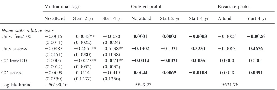
Home state relative costs:
Univ. fees/100 20.0015 0.0045** 20.0030 0.0001 0.0002 20.0003 20.0005 20.0026
(0.0011) (0.0022) (0.0024)
Univ. access 20.0487 20.4651** 0.5138** 20.1302 20.1931 0.3233 20.0063 0.4676
(0.0451) (0.0980) (0.1038)
CC fees/100 0.0006 20.0077** 0.0071** 20.0014 20.0021 0.0035 0.0000 0.0005
(0.0012) (0.0032) (0.0032)
CC access 20.0099 0.0514 20.0415 0.0044 0.0065 20.0108 0.0018 0.0391
(0.0590) (0.1237) (0.1356)
Log likelihood 256190.16 25849.23 25631.76
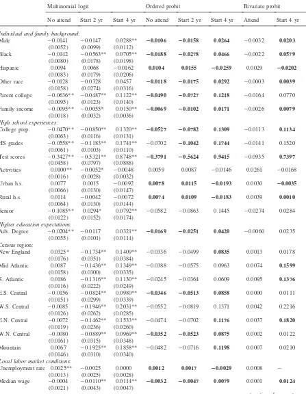
a Notes: Marginal effects are the derivatives of the probability function evaluated at the sample means for continuous variables, and the difference between 0 and 1 for dummy variables. Standard errors in parentheses. Values inboldlie within the 95% confidence interval around the estimated marginal effects for the multinomial logit.
marginal effects compare between the three models. To do this, we calculate confidence intervals around the esti-mated multinomial logit marginal effects and ask whether the estimated ordered and bivariate probit mar-ginal effects lie within that interval. If so, we conclude that the models provide similar estimates, which are reported in bold type in Table 3. If not, we conclude that the marginal effects are not statistically similar. Note that the first marginal effects for the bivariate probit represent the marginal effects for the attendance/non-attendance decision and are not directly comparable to the marginal effects in the other two models for the non-attendance and 2-year attendance decisions.
Table 3 suggests that the results of the three models are generally quite consistent. In nearly all cases, the estimated marginal effects for the ordered probit and the decision to attend a 4-year college for the bivariate probit are within the 95% confidence interval of the marginal effects from the multinomial logit model. Exceptions occur for the effect of extracurricular activities, the effect of belonging to the senior cohort, and the relative effect of living in several of the census region instead of the Pacific region. This general statistical agreement between models is comforting, especially for the key variables that researchers usually study, as it suggests that our estimates and therefore our conclusions are not driven solely by our choice of specification and more-over that the choice of specification does not appear to greatly affect our conclusions.
The estimated marginal effects in Table 3 are consist-ent with previous findings. In interpreting these results, recall that the students being studied are those who reported as seniors in high schools that they expected to receive at least a Bachelor’s degree. Controlling for fam-ily background and measured academic ability, males are significantly more likely than females to attend 4-year
colleges while Blacks are significantly more likely than whites to attend 4-year colleges and significantly less likely to attend 2-year colleges (similar to Hilmer, 1997). As with (Behrman, Rosenzweig, & Taubman, 1996; Kane, 1994), students from families with higher parental education and income are significantly more likely to attend 4-year colleges and less likely to either attend 2-year colleges or not attend at all. Similar patterns are observed for students following college preparatory pro-grams and receiving higher grades and test scores (Hilmer, 1998; Ganderton, 1992). For each of those vari-ables, the estimated marginal effects are largest for the 4-year college option, suggesting that students likely base their decision to initially invest in a higher priced 4-year college than a lower priced 2-year college on the important signal provided by measured ability and aca-demic performance. As would be expected, students expecting to receive an advanced degree are significantly more likely to attend a 4-year college and significantly less likely to attend neither type of college. Finally, it appears that students from the Pacific region are signifi-cantly more likely than students from the remaining regions to attend 2-year colleges and significantly less likely to attend 4-year colleges. This is not at all surpris-ing as California and Arizona boast two of the largest community college systems in the United States.
student is to directly enter a 4-year college (Brewer et al., 1999). As with Hilmer (1998) there appear to be positive cross-price effect between 2- and 4-year col-leges as increase in 2-year fees increase the likelihood of 4-year attendance while increase in 4-year fees increase the likelihood of 2-year attendance. As the same time, the expected negative own price effects (e.g. Kane, 1994; Parker & Summers, 1993; Leslie & Brinkman, 1987; Heath & Tuckman, 1987; Chressanthis, 1986) are observed for both 2- and 4-year colleges but is only sig-nificant for the former. Finally, within this sample, only the relative access of 4-year college significantly affects students decisions with students living in states with rela-tively more 4-year colleges being significantly more likely to attend 4-year colleges and significantly less likely to attend 2-year colleges.
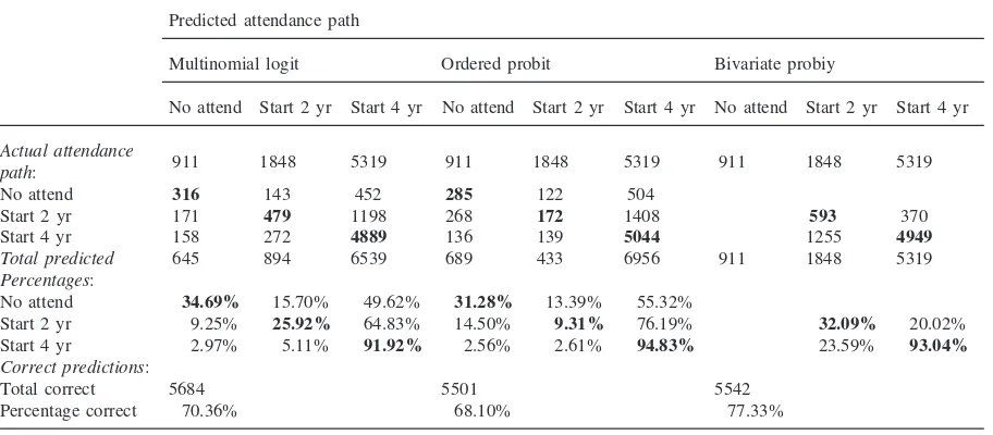
An important concern with such models is the degree to which they correctly predict actual student attendance decision. To get some idea how the three models com-pare over this measure, Table 4 presents predicted and actual attendance decisions for each of the three models. Note, because we estimate the bivariate probit with sam-ple selection, non-attendance is predicted perfectly and actual and predicted choices are only observed for the 2- and 4-year options. Looking first at the total percent correct predictions the models correctly predict a stud-ent’s college choice roughly 70% of the time. These values compare favorably with the 61% correct predic-tions for the multinomial logit estimated in Brewer et al. (1999) for a sample of HSB students that was deemed by the authors to “do a reasonable job of predicting an
Table 4
Comparison of predicted and actual attendancea
Predicted attendance path
Multinomial logit Ordered probit Bivariate probiy
No attend Start 2 yr Start 4 yr No attend Start 2 yr Start 4 yr No attend Start 2 yr Start 4 yr
Actual attendance
911 1848 5319 911 1848 5319 911 1848 5319
path:
No attend 316 143 452 285 122 504
Start 2 yr 171 479 1198 268 172 1408 593 370
Start 4 yr 158 272 4889 136 139 5044 1255 4949
Total predicted 645 894 6539 689 433 6956 911 1848 5319
Percentages:
No attend 34.69% 15.70% 49.62% 31.28% 13.39% 55.32%
Start 2 yr 9.25% 25.92% 64.83% 14.50% 9.31% 76.19% 32.09% 20.02%
Start 4 yr 2.97% 5.11% 91.92% 2.56% 2.61% 94.83% 23.59% 93.04%
Correct predictions:
Total correct 5684 5501 5542
Percentage correct 70.36% 68.10% 77.33%
a Notes: Values inboldrepresent predicted decisions that agree with actual decisions. Because non-attendance is predicted perfectly for the bivariate probit, total correct decisions are only calculated for the 2- and 4-year attendance decisions and the percentage correct is compared to the total number of 2- and 4-year attendees, 7167, rather than the total number of students in the sample, 8078. individual’s choice of college.” Turning to how the cor-rect predictions differ across paths, all three models are remarkably successful at predicting 4-year college attendance, correctly predicting that decision more than 90% of the time. Conversely, the models are not very successful at predicting non- and 2-year attendance, cor-rectly predicting those decisions roughly one-third, and less than one-quarter of the time, respectively.
As a final part of this exercise, we want to examine whether choice of specification affects the results of the now popular two-stage corrections for selectivity bias that estimate the college attendance equation as the first stage (e.g. Brewer et al., 1999; Hilmer, 1997; Ganderton, 1992). The application used here applies to estimating the number of years of college that a student completes dependent on the type of institution he or she initially attends.15 Such estimation is a classic example of the
potential for self-selection bias, as students the decision to attend either a 2- or a 4-year college is a non-random decision. This is potentially problematic for the follow-ing reason. To correctly estimate whether there is a dif-ference in the years of college completed by 2- and 4-year attendees who expect to graduate, we would like to choose a student who expects to graduate at random,
send him or her to a 2-year college, send him or her to a 4-year college, and observe the difference. However, due to the non-randomness of student attendance decisions, simply estimating years of college completed functions for the subsets of students who attended 2- and 4-year colleges would not repeat that desired experiment. For example, suppose there were some negative years of college effect associated with 2-year college attendance. Estimation based on regular OLS would predict equal years completed for students who are identical in every observable way except for 2- and 4-year college attend-ance although in reality due to the negative 2-year col-lege effect students at the 2-year colcol-lege would actually complete fewer years.
An important concern in estimating such two-stage systems is identification. For the system to be identified, we must make an identifying restriction by including at least one variable in the first-stage attendance equation that is not included in the second stage persistence func-tions. Ideally, this restriction should be economically jus-tifiable. Our solution is to include state-specific relative cost measures (representing the direct costs of tuition and fees and the indirect costs of relative access to different types of institutions in the student’s home state in 1982)16in the attendance path estimation but not the
per-sistence functions. The use of state-level average tuition as an instrument is reasonable as these values measure the relative costs of attending different types of insti-tutions. Presumably, the relative attendance costs at dif-ferent types of in-state institutions only affect student decisions among different potential initial institutions and not their persistence decisions once at the initial institution (which should be affected by the direct attend-ance cost at that particular institution). Rouse (1995) uses a similar argument to justify the use of distance to the nearest community college and university as an instru-ment for college attendance. Namely, a student’s dis-tance from those postsecondary institutions, like average in-state attendance costs, proxies for the relative cost of attending different institutions which affects the initial attendance decision but not the persistence decision.
Table 5 presents the results of estimating the years of college completed functions by regular OLS and by selectivity-corrected OLS using each of the three speci-fications of the college attendance equation to generate the first-stage estimates. As with most previous studies, the results suggest that the selectivity-corrected results outperform the regular OLS results. Comparing across the selectivity-corrected results suggests that choice of specification may affect the conclusions that can be
16 We use data from 1982 because that is the year that sopho-mores in the HSB graduated from high school and thus the year in which they would be making their initial college attend-ance decision.
drawn from this type of model. For 4-year college atten-dees, the coefficient estimates tend to be higher for the ordered probit than the coefficient estimates for the remaining models, which themselves are generally quite similar. A potentially more troubling difference is that the estimated effect of test scores on the years of college completed is only significant for the ordered probit and not for the multinomial logit and bivariate probit. As the effect of measured academic ability on college persist-ence may be an important policy concern for states con-sidering increasing admission standards at 4-year insti-tutions; this difference is a potentially serious concern in the choice of specification. Turning to 2-year attendees, the most prominent difference between the multinomial logit and ordered probit is that parental education, family income, high school program, and high school grades are only estimated to be significant for the multinomial logit. While statistical significance is a matter of degree, most researchers draw conclusions based only on variables estimated to be statistically significant, which suggests that the conclusions drawn from the two models might be quite different. Moreover, the sizes of the estimated coefficients for the two models differ a great deal for many of the independent variables. These potential dif-ferences are much greater for 2-year attendees than 4-year attendees and may result from the fact that as dem-onstrated in Table 4 the three statistical models are much more successful at predicting 4-year attendance than 2-year attendance.
selectivity-correc-Table 5
Estimated OLS and selectivity corrected effects of selected characteristics on years of college completeda
OLS Multinomial probit Ordered probit Bivariate
Start 2 yr Start 4 yr Start 2 yr Start 4 yr Start 2 yr Start 4 yr Start 4 yr
Individual and family background:
Male 0.0303 0.0330 0.0400 0.0249 0.0193 0.0425 0.0342
(0.0635) (0.0335) (0.0644) (0.0350) (0.0730) (0.0355) (0.0341) Black 20.2514** 20.0936 20.2647** 20.0860 20.2707** 20.0793 20.0751 (0.1105) (0.0649) (0.1005) (0.0535) (0.1174) (0.0555) (0.0657)
Hispanic 0.0964 20.1360* 0.0824 20.1250** 0.1084 20.1623** 20.1384*
(0.1036) (0.0736) (0.0861) (0.0536) (0.0953) (0.0560) (0.0747)
Other race 0.2602 0.0342 0.2535* 0.0303 0.2501* 0.0431 0.0039
(0.1666) (0.1027) (0.1312) (0.0783) (0.1338) (0.0782) (0.0103) Parent college 0.1422* 0.1841** 0.2023** 0.1455** 0.0932 0.2307** 0.1794**
(0.0785) (0.0374) (0.0884) (0.0458) (0.1765) (0.0528) (0.0469)
Family income 0.0245 0.0289** 0.0363* 0.0218* 0.0182 0.0364** 0.0257**
(0.0204) (0.0112) (0.0209) (0.0117) (0.0291) (0.0124) (0.0123) High school experiences:
College prep. 0.2833** 0.2157** 0.3218** 0.1940** 0.2329 0.2778** 0.2337** (0.0678) (0.0437) (0.0709) (0.0469) (0.1770) (0.0650) (0.0543)
HS grades 0.2343** 0.5269** 0.2707** 0.5083** 0.1659 0.6060** 0.5536**
(0.0564) (0.0321) (0.0596) (0.0341) (0.2275) (0.0660) (0.0514)
Test scores 0.4271 0.5392* 0.6903 0.3344 0.0476 0.9825** 0.5697
(0.4725) (0.2839) (0.4792) (0.2956) (1.2955) (0.4239) (0.3742)
Activities 0.0165 20.0124 20.0024 20.0030 0.0221 20.0187 20.0688
(0.0179) (0.0096) (0.0210) (0.0117) (0.0251) (0.0115) (0.1071) Urban h.s. 20.0179 20.1898** 20.0408 20.1778** 20.0119 20.1975** 20.1787**
(0.0823) (0.0450) (0.0809) (0.0449) (0.0819) (0.0448) (0.0457)
Rural h.s. 0.2126** 20.0150 0.1684* 0.0084 0.2145** 20.0173 0.0046
(0.0839) (0.0407) (0.0924) (0.0468) (0.0914) (0.0455) (0.0422)
Senior 0.3792** 0.6724** 0.5605** 0.5761** 0.3248 0.7307** 0.6204**
(0.0921) (0.0542) (0.1343) (0.0777) (0.2008) (0.0719) (0.0726) Higher education expectations:
Adv. degree 0.0358 20.0241 0.0582 20.0379 0.0185 20.0085 20.0284
(0.0644) (0.0338) (0.0658) (0.0359) (0.0840) (0.0370) (0.0353) Census region:
New England 0.0145 0.2764** 20.1832 0.3551** 20.0584 0.3488** 0.0445** (0.1656) (0.0776) (0.2122) (0.0951) (0.2972) (0.0996) (0.0121)
Mid Atlantic 0.2730** 0.2828** 0.1685 0.3249** 0.2008 0.3572** 0.4347**
(0.1102) (0.0671) (0.1243) (0.0695) (0.2609) (0.0854) (0.1098)
S. Atlantic 0.1615 0.2364** 0.0788 0.2752** 0.1292 0.2717** 0.3676**
(0.0991) (0.0704) (0.1055) (0.0727) (0.1381) (0.0749) (0.1003) E.S. Central 20.0313 20.2697** 20.0811 20.2535** 20.0776 20.2204** 20.0142 (0.1483) (0.0935) (0.1643) (0.1019) (0.2266) (0.1093) (0.0119) W.S. Central 20.0162 20.1253* 20.0858 20.0862 20.0713 20.0604 0.0241
(0.1223) (0.0754) (0.1296) (0.0763) (0.2206) (0.0882) (0.1136)
E.N. Central 0.1569 0.1748** 0.0662 0.2133** 0.0963 0.2401** 0.3255**
(0.1007) (0.0656) (0.1143) (0.0680) (0.2229) (0.0815) (0.1077)
W.N. Central 0.1764 0.2529** 0.1039 0.2783** 0.1111 0.3254** 0.0390**
(0.1395) (0.0783) (0.1677) (0.0840) (0.2723) (0.0983) (0.0113) Mountain 20.6783** 20.2191** 20.7926** 20.1759* 20.7271** 20.1608 20.0071 (0.1735) (0.1003) (0.2041) (0.1046) (0.2527) (0.1113) (0.0130)
Table 5 (continued)
OLS Multinomial probit Ordered probit Bivariate
Start 2 yr Start 4 yr Start 2 yr Start 4 yr Start 2 yr Start 4 yr Start 4 yr
Selectivity correction terms:
l1 2 2 0.9620** 20.6076** 20.1472 0.3390 0.1695
– – (0.4681) (0.2997) (0.4782) (0.2366) (0.5682)
l2 – – – – – – 0.4394*
– – – – – – (0.3872)
R2 0.1006 0.1982 0.1027 0.1988 0.1007 0.1985 0.1987
a Notes: Sample sizes are 1848 and 5319, respectively for 2- and 4-year attendees. Estimation also includes dummy variables that are equal to one if values for a variable are missing (in which case those variables are set to zero). Data are weighted. Standard errors in parentheses. *, ** Significant at the 5 and 10% levels.
tion terms are significant for both groups of students, the ordered probit estimates the terms to be significant for neither group of students, while the bivariate probit esti-mates the terms to be significant only for the decision to attend a 4-year college.
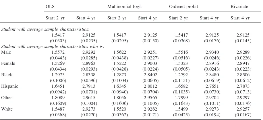
The final part of this exercise is to explore whether the cross-specification differences in the selectivity-cor-rected years of college completed functions outlined above lead to differences in the predicted years of col-lege completed by different students. Table 6 presents predicted years of college completed for students pos-sessing average sample characteristics for all values except gender and ethnicity, which are varied to generate predicted values for a hypothetical average student
Table 6
Predicted years of college completed for average studentsa
OLS Multinomial logit Ordered probit Bivariate
Start 2 yr Start 4 yr Start 2 yr Start 4 yr Start 2 yr Start 4 yr Start 4 yr
Student with average sample characteristics:
1.5417 2.9125 1.5417 2.9125 1.5417 2.9125 2.9125
(0.0303) (0.0235) (0.0295) (0.0150) (0.0368) (0.0176) (0.0145) Student with average sample characteristics who is:
Male 1.5572 2.9292 1.5622 2.9251 1.5516 2.9340 2.9289
(0.0443) (0.0285) (0.0438) (0.0227) (0.0516) (0.0246) (0.0226)
Female 1.5269 2.8963 1.5222 2.9003 1.5323 2.8916 2.8947
(0.0434) (0.0293) (0.0428) (0.0224) (0.0505) (0.0243) (0.0223)
Black 1.2973 2.8338 1.2873 2.8402 1.2792 2.8480 2.8506
(0.1006) (0.0596) (0.1004) (0.0605) (0.1151) (0.0619) (0.0612)
Hispanic 1.6451 2.7913 1.6345 2.8012 1.6582 2.7651 2.7873
(0.0942) (0.0701) (0.0940) (0.0704) (0.1035) (0.0730) (0.0713)
Other 1.8089 2.9615 1.8056 2.9565 1.7999 2.9704 2.9297
(0.1609) (0.1004) (0.1606) (0.1005) (0.1643) (0.1011) (0.0176)
White 1.5487 2.9273 1.5520 2.9262 1.5499 2.9273 2.9257
(0.0368) (0.0270) (0.0362) (0.0171) (0.0425) (0.0194) (0.0167)
attendance equation in two-stage selectivity-correction models. Analyzing the values suggest that among both 2- and 4-year attendees, males are predicted to complete slightly more years of college than females. Black 2-year attendees are predicted to complete significantly fewer years than 2-year attendees from the remaining ethnic groups. At the same time, Black 4-year attendees are pre-dicted to complete more years than Hispanics and only one-tenth of a year fewer years than whites and Other race students.
5. Conclusion
This paper estimates the college attendance equation as a multinomial logit, an ordered probit, and a bivariate probit with sample selection and compares the results to examine whether choice of specification affects the estimated parameters. It is important to stress that the results above only directly apply to the data analyzed and the attendance decision modeled. Nonetheless, the results do provide some indication of the potential importance of carefully considering specification issues before estimating the college attendance equation for some applications. Overall, the results suggest the esti-mated marginal effects generally do not differ signifi-cantly across specifications, suggesting that choice of specification may not make that much difference for the college attendance decision itself. However, extending the analysis to two-stage selectivity-correction models suggests that choice of specification might, at least for some applications, affect the estimated significance of different independent variables and the predicted out-comes based on those estimates.
A less-than-desirable feature of the simple specifi-cation tests employed above is that they can only be used to test whether a specification itself is appropriate and not which appropriate specifications are superior to others. This is because most traditional specification tests are based on comparing models that can be nested and then directly compared. Unfortunately, the models dis-cussed above cannot be nested and therefore such approaches do not work. Following recent advances in statistical techniques, it might be possible to perform some type of non-nested test to try and determine the superior specification of the college attendance equation. This might be an approach that researchers would like to explore in the future.
References
Behrman, J. R., Rosenzweig, M. R., & Taubman, P. (1996). College choice and wages: estimates using data on female twins.Review of Economics and Statistics,78(4), 672–685. Brewer, D., Eide, E., & Ehrenberg, R. G. (1999). Does it pay
to attend an elite private college? Cross cohort evidence on the effects of college quality on earnings.Journal of Human Resources,34(1), 104–123.
Broomhall, D. E., & Johnson, T. G. (1994). Economic factors that influence educational performance in rural schools. American Journal of Agricultural Economics,76, 557–567. Chressanthis, G. A. (1986). The impacts of tuition rate changes on college undergraduate headcounts and credit hours over time: A case study. Economics of Education Review, 5, 205–217.
Evans, W. N., & Schwab, R. M. (1995). Finishing high school and starting college: Do catholic schools make a difference? Quarterly Journal of Economics,110(4), 941–974. Ganderton, P. T. (1992). The effect of subsidies in kind on the
choice of a college. Journal of Public Economics, 48, 269–291.
Greene, W. H. (1997).Econometric Analysis.(3rd ed.). Engle-wood Cliffs, NJ: Prentice–Hall.
Greene, W. H. (1998).Limdep 7.0 user’s manual. Econometric Software, Inc.
Gyourko, J., & Tracy, J. S. (1988). An analysis of public- and private-sector wages allowing for endogenous choices of both government and union status.Journal of Labor Eco-nomics,6, 229–253.
Hausman, J., & McFadden, D. (1984). Specification tests for the multinomial logit model.Econometrica,52(5), 1219–1240. Heath, J. A., & Tuckman, H. P. (1987). The effects of tuition level and financial aid on the demand for undergraduate and advanced terminal degrees.Economics of Education Review, 6, 227–238.
Heckman, J. (1979). Sample selection bias as a specification error.Econometrica,47, 153–161.
Hilmer, M. J. (1998). Post-secondary fees and the decision to attend a university or a community college.Journal of Pub-lic Economics,67, 329–348.
Hilmer, M. J. (1997). Does community college attendance pro-vide a strategic path to a higher quality education? Econom-ics of Education Review,16(1), 59–68.
Kane, T. J. (1994). College entry by blacks since 1970: The role of college costs, family background, and the returns to education.Journal of Political Economy,102, 878–911. Kennedy, P. (1998).A Guide to Econometrics.(4th ed.).
Cam-bridge, MA: MIT Press.
Lee, L. F. (1983). Generalized econometric models with selec-tivity.Econometrica,51, 507–512.
Leslie, L. L., & Brinkman, P. T. (1987). Student price response in higher education. Journal of Higher Education, 58, 181–204.
Maddala, G. S. (1983).Limited dependent and qualitative vari-ables in econometrics. Cambridge: Cambridge University Press.
National Center for Education Statistics (1987)High school and beyond 1980 senior cohort third follow-up (1986) volumes I and II: Data file users manual. Washington, DC: US Department of Education.
Office of Educational Research and Improvement (1997). Digest of educational statistics. Washington DC: US Department of Education.
vocational education. Economics of Education Review, 14 (4), 335–350.
Parker, J., & Summers, J. (1993). Tuition and enrollment yield at selective liberal arts colleges.Economics of Education Review,12, 311–324.
Rouse, C. E. (1995). Democratization or diversion? The effect of junior colleges on educational attainment. Journal of Business and Economic Statistics,13, 217–224.
Savoca, E. (1991). The effect of changes in the composition of financial aid on college enrollments.Eastern Economic Journal,17(1), 109–121.