20
The Effect of Water Level on The Effectiveness
of Sediment Flushing
Pranoto Samto Atmodjo and Suripin Civil Eng Department of Diponegoro University Jl. Prof. Sudarto SH No 1 Tembalang, Semarang - Indonesia
e-mail: [email protected]
Abstract - This research is focused on determining the effective flushing water level in pressure flushing activity at storage
sedimen based on the hydraulic physical model test in the laboratory. The effective water level is the elevation of water level in sediment flushing which result in the highest concentration of sediment scours. Effective flushing water level is the elevation of water level near the top layer of sediment deposit which can trigger the erosion of the top layer of sediment so that it creates a maximum scours. That elevation is known as Effective Flushing Water Level (EFWL). This research was conducted in the laboratory using Wonogiri Reservoir prototype, with scale model of 1:66.67. The model operated without inflow, started from control water level (CWL) .and lowered gradually by operating the flushing gates. The gates were operated of a = 2.50 cm. The flushing implementation was repeated with variation of sediment thickness Hs=1.50; 3.00; 3.75 and 4.50 cm. The water level, sediment concentration, flushing discharge, and the flow velocity in the upstream of the gates were observed every 1.50 cm lowered of water level. Coal dust was used in this research to substitute sediment material. This research found that the effective watel level (Hef) is function of sediment thickness (Hs) in from of :
= 10.58 . , and the sediment concentration is related with scour parameters in the form of :
=
. . . .
where ,Cmo: sediment concentration source model (mg/l), Qw: f lushing discharge (m³/dt), Hs : sediment thickness (m), v : flow velocity (m/dt), Hw: water depth (m). The result of this research is expected to be used as an initial consideration of effective sediment flushing in Wonogiri reservoir protoype in order to reduce the capacity loss of the reservoir due to sedimentation , or in other words to extend the life time plan of reservoir.
[Keywords : sedimentation; effective water level; sediment flushing]
Submission: September 20, 2012 Accepted : December 21, 2012
INTRODUCTION
Dam in the form of reservoir has several functions, such as: flood control, power plant, irrigation, water supply, and others. River damming will reduce flow rate, and consequently, carried sediment will settle, and decrease the reservoir capacity.
Most of the dam are planned and operated for a certain age, that is, because –mostly- there is the accumulation of sediment, instead of due to construction damage (Morris and Fan, 1998). Therefore, if the occurrence of sedimentation rate is larger than the sedimentation rate design, the age of the reservoir will be shorter than the plan.
Commonly, in Indonesia, the sedimentation rate which goes into the reservoir is quite high. For example: in Wonogiri Reservoir, the rate of capacity reduction because of the sedimentation is averagely 2.70 % per year (JICA, 2007), in Mrica Reservoir: 2.60 % per year (Soewarno and Syariman, 2008), Sempor: 1.64 % (Sinaro et al., 2002). This case is high enough compare to the rate of reservoir capacity reduction on the world because sedimentation, which is averagely 1% (Yoon, 1992).
Efforts to reduce the decrease of reservoir capacity because of the sedimentation, among others is preventing sediment inflow into the reservoir, that is,
by controlling upstream area, for example: upstream conservation, check dam construction, to build a divertion channel. Another effort is by remove the sediment which has already been in or settled inside the reservoir, namely, by Hydraulic Flushing and
dredging.
There are 3 kinds of way of hydraulic flushing, that is: Sluicing Operation, venting of density current, and flushing operation. Sluicing operation is an removing by controlling the inflow sediment inside the reservoir so that it will not quickly settle, by lowering the reservoir water surface. Sluicing is usually done during the flood. Venting is controlling the capacity of sediment so that it will not settle, and continuously removing through the bottom gate of the reservoir without lowering the reservoir water surface. On the other hand, flushing is aimed to flush the sediment which has already settled in the bottom of the reservoir. This operation technique is established by increasing the flow rate in the flushing gate, so that the rate inside the reservoir is larger and enough to erode the sediment which has accumulated through the flushing gate system (for instance: bottom outlet system) (Meskhati et al., 2009).
21 drainage and reached the free flow condition (White
and Bettes, 1984) but in this case, it must sacrifice the water storage in the reservoir (Yang, 1996). Flushing can be applied without lowering the reservoir water surface or in the high water surface (Morris and Fan, 1998). The application of flushing with high water surface (pressure flushing) is more frequently conducted to avoid reservoir emptying. From the available references, there is no source which explicitly explained in what height the water will produce the most effective sediment flushing.
This research focused on the flushing of high water surface or pressure flushing to know in what height the water surface will produce the most effective flushing from variations of sediment thickness by physical hydraulic test in laboratory.
Modeling the mechanism of sediment flushing in reservoir by operating the gate to know the height of water surface which produce the most effective sediment scours. It is expected by knowing the matter above, so that it can be used to reduce the rate of the reservoir capacity reduction because of sedimentation, or it can elongate the age of reservoir plan by sediment flushing.
The scope of this study includes physical hydraulic model test on the sediment pressure flushing in reservoir according to the result of Nippon Koei Co., LTD, 2009 design.
The scopes of the study are as follows:
1. The making of Physical Model based on the initial plan.
2. The research of discharge inflow to obtain discharge curve, rate of pattern and distribution from several discharge variations in the model
3. The measurement of Sediment Concentration which comes out of the reservoir in each water surface reduction, one meter of every sediment thickness variation
4. Determining what height of water surface which is the most effective in flushing application.
The limitations of the study include:
1. Sediment thickness variation for the testing 1.50; 2.25; 3.00; 3.75 and 4.50 cm
2. Collecting the data variable Q,V,C,L, in the interval of water surface reduction every 1.50 cm, and the height of maximum water surface of 13.95 cm. 3. Gate opening remains constant 2.50 cm
4. No water discharge entering the reservoir during the application of flushing
Some early researchers have done a study about sediment flushing, for instance:
Fan and Jiang (1980), developed an empirical formula based on the research in Sanmenxia Reservoir in China. The formula linked between: sediment discharge which comes out of the reservoir is the function from the width of the bottom of the channel and discharge as follows:
= 0.00035 . ( 10 ) . . The research
was conducted between the year of 1963 and 1964. The
diameter which was flushed during the operation was between 0.06-0.09 mm.
Xia (1983) delivered the formula of the amount of sediment discharge as the functions of the slope of the channel base, the amount discharge of coming out, the width of the channel, and the value of soil erodibility, as follows:
=
. .
. , the bigger the soil erodibility value, the easier the sediment erode, it shows the sediment material which can be easily eroded. On the other hand, the low coefficient value of erodibility indicates the material of sediment which is rough or consolidated.
Scheuerlein (1993) analyzed theoretically the height of effective water surface in sediment flushing based on hydraulic in pressure flushing. Pressure flushing with drawdown based on two continuous stages. On the first stage, in which the water pressure is still high, there is retrogressive erosion, and on the next stage, where the low water pressure near with the surface layer of sediment, there is progressive erosion. The height of the effective water surface happens on the condition of progressive erosion, as in Figure.1.
Figure.1 Pressure Flushing
Figure.1 Height Water Level Flushing (Pressure flushing)
The height of effective water surface: = ( )+ ...(1)
From the early researchers, there isn’t any empirical research which revealed what is the effective height of water surface in sediment flushing.
METODOLOGY
Physical Hydraulic Test
22 research is conducted by using Physical Hydraulic
Model Test in laboratory. Model Situation and Material
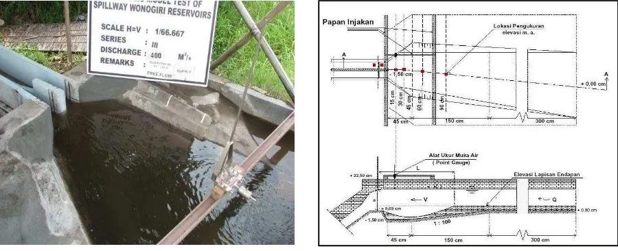
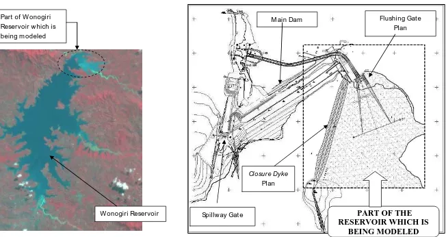
The situation and part of reservoir prototype condition which will be modeled is as in Figure.2. The reservoir model created consists of some storage, Closure Dyke, spillway, and flushing gate, photo and plan of model as in Figure.3. Imitation material of the sediment used is coal dust.
Test Scenario
This test scenario involves sequences of test stages, location and types of observation, test variation and planning of data obtained. There are 3 series of test scenario, they are:
1.Series 0: To test the capacity of flushing gate, and flow pattern from the initial design.
2.Series 1: To test several variations of gate opening, discharge, and sediment thickness.
3.Series 3: To determine the elevation of effective water surface in the application of flushing
In the series 0 test which has been conducted, the result is that the capacity of flushing gate is able to flows the discharge as design, which is able to pass discharge Q=11.05 l/s with water surface elevation under +19.50 cm, or equal as the prototype 400 m3/s, elevation +140.00 m.
In the series 2 test which has been conducted, it produced the shape of upper course wing of 45o flow pattern is better in the wing angle of 90o, and gate opening a=2.50 cm or in the prototype is 1.67 m is the most effective compare to the other opening which has been attempted 1.15 and 5.30 cm.
For the next research (Series 2) is used the opening gate of 2.50 cm, and upper course wing of 45o with test scenario as in Table1.
a.Flushing Gate b. Plan and the Long section of Flushing Gate
Figure.2. Photo and Plan of the Model Table 1. Test Scenario
Series/
Stages
Location of
Observation Items of Observation Types/ variation of test The results obtained
Series 2 Upper course Intake Area
(with sediment) Qin=0 l/s, Water surface gets lowering every 1.50 cm
1. The relation of discharge and upstream water surface
2. Time of reduction m.a every 1.50 cm 3. Length of scours every
m.a lower 1.50 cm 4. Sediment
concentration coming out of the reservoir every m.a lower 1.50 cm
Qin= 0 (no discharge coming
in), the initial water surface of the reservoir =13.95 cm, then water level is lowered with gate opening 2.50 cm, and take the data every lowering 1.50 cm. Running is conducted repeatedly for sediment variation of: 1.50; 2.25; 3.00; 3.75; 4.50 cm
Running with gate opened a = 2.50 cm: 1.Relation of discharge and height of
water level
2.Time every water level lowered 1.50 cm
3. Rate/Length of scours
4. Sediment concentration coming out of the reservoir
23 Figure 3. Wonogiri Reservoir and Part of the Reservoir which is being modeled
Spillw ay Gat e
Closure Dyke Plan
M ain Dam
PART OF THE
RESERVOIR WHICH IS
BEING MODELED
Flushing Gat e Plan
Wonogiri Reservoir Part of Wonogiri
24 RESULT OF THE ANALYSIS AND DISCUSSION
Result
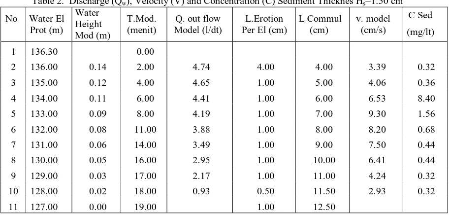
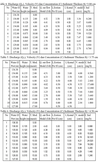
Modeling with opening gate stays 2.50 cm, with observation and measurement includes height of the water surface (Hw), time (T), discharge (Qw), velocity (V), dan concentration (C). Those measurements above is established in every 1.50 cm reduction of water surface starting from 13.50 cm elevasion or the same as +136.00 m in the prototype, and it is repeated on each sediment thickness variation Hs=1.50; 2.25; 3.00; 3.75; 4.50 cm, without any discharge coming into the reservoir. Result of the observation is as in Table2 until Table 6 and Figure.3 until 6.
Dimensional Analysis
Dimensional analysis helps reducing the similarity stated in undimensional parameter to concern with the relative significance on each parameter. In physical modeling, it
can process the result of the experiment in forms of sistematically undimensional parameter.
From the application of flushing, the influencing variables are:
Hw, g, ρw, Qw, Hs,ds, ρs , C, v
In which : Hw= height of water surface (m), g = gravity (m/s2), ρw = water mass density (mg/l), Qw = water discharge (m3/dt), Hs = sediment thickness (m),
ds= average sediment diameter (m), ρs = sediment mass density (mg/l), C = concentration of sediment eroded (mg/lt), dan v= flow velocity (m/s)
After selected based on M, L, and T dimension, and analyzing the result:
= .
. , , if (Constanta) is emitted, therefore:
= .
.
Table 2. Discharge (Qw), Velocity (V) and Concentration (C) Sediment Thicknes Hs=1.50 cm No Water El
Prot (m)
Water Height Mod (m)
T.Mod. (menit)
Q. out flow Model (l/dt)
L.Erotion Per El (cm)
L Commul (cm)
v. model (cm/s)
C Sed (mg/lt)
1 136.30 0.00
2 136.00 0.14 2.00 4.74 4.00 4.00 3.39 0.32
3 135.00 0.12 4.00 4.65 1.00 5.00 4.06 0.36
4 134.00 0.11 6.00 4.41 1.00 6.00 6.53 8.40
5 133.00 0.09 8.00 4.19 1.00 7.00 9.30 1.56
6 132.00 0.08 11.00 3.88 1.00 8.00 8.20 0.68
7 131.00 0.06 14.00 3.49 1.00 9.00 7.50 0.44
8 130.00 0.05 16.00 2.95 1.00 10.00 6.41 0.44
9 129.00 0.03 17.00 2.17 1.00 11.00 4.24 0.32
10 128.00 0.02 18.00 0.93 0.50 11.50 2.93 0.32
11 127.00 0.00 19.00 1.00 12.50
Table 3. Discharge (Qw), Velocity (V) dan Concentration (C) Sediment Thicknes Hs=2.25 cm
No Water El Water T. Mod. Q. out flow L.Erotion L Komul V. model C Sed Prot (m) height (m) (menit) Model (l/dt) Per El (cm) (cm) (cm/s) (mg/lt)
1 136.30 0.00
2 136.00 0.135 2.00 4.52 4.00 4.00 3.42 0.88
3 135.00 0.120 4.00 4.43 0.50 4.50 4.06 1.04
4 134.00 0.105 6.00 4.31 0.50 5.00 5.40 1.20
5 133.00 0.090 8.00 4.12 0.50 5.50 9.42 11.12
6 132.00 0.075 11.00 3.80 0.50 6.00 8.05 5.20
7 131.00 0.060 14.00 3.40 0.50 6.50 7.66 4.72
8 130.00 0.045 16.00 2.95 0.50 7.00 6.65 2.72
9 129.00 0.030 17.00 2.10 0.50 7.50 3.87 1.44
10 128.00 0.015 18.00 0.88 0.50 8.00 2.71 1.36
25 Table 4. Discharge (Qw), Velocity (V) dan Concentration (C) Sediment Thicknes Hs=3.00 cm
Table 5. Discharge (Qw), Velocity (V) dan Concentration (C) Sediment Thicknes Hs= 3.75 cm
Table 6. Discharge (Qw), Velocity (V) dan Concentration (C) Sediment Thicknes Hs= 4.50 cm
No
Water El
Water T. Mod. Q. out flow L.Erotion
L Komul V. model C Sed
Prot (m) height (m) (menit)
Model (l/dt) Per El (cm)
(cm)
(cm/s) (mg/lt)
1
136.30
0.00
2
136.00
0.135
2.00
4.52
3.50
3.503.36
0.240
3
135.00
0.120
4.00
4.41
0.50
4.003.87
0.680
4
134.00
0.105
6.00
4.19
0.50
4.505.25
0.920
5
133.00
0.090
8.00
4.09
0.50
5.009.33
18.280
6
132.00
0.075
10.00
3.88
0.50
5.507.99
9.520
7
131.00
0.060
12.00
3.49
0.50
6.007.47
3.000
8
130.00
0.045
13.00
2.78
0.00
6.006.65
1.800
9
129.00
0.030
14.00
2.03
0.50
6.503.75
0.880
10
128.00
0.015
15.00
0.84
0.00
6.502.78
0.760
11
127.00
16.00
0.50
7.00No Water El Water T. Mod. Q. out flow L.Erotion L Komul V. model C Sed Prot (m) height (m) (menit) Model (l/dt) Per El (cm) (cm) (cm/s) (mg/lt)
1 136.30 0.00
2 136.00 0.135 2.00 4.51 3.00 3.00 4.00 0.560
3 135.00 0.120 4.00 4.33 0.50 3.50 5.00 1.200
4 134.00 0.105 6.00 4.22 0.50 4.00 5.83 2.880
5 133.00 0.090 8.00 4.02 0.50 4.50 9.55 17.600
6 132.00 0.075 10.00 3.68 0.50 5.00 8.30 12.080
7 131.00 0.060 12.00 3.25 0.50 5.50 7.84 5.080
8 130.00 0.045 13.00 2.70 0.00 5.50 7.05 3.640
9 129.00 0.030 14.00 1.59 0.50 6.00 4.30 2.400
10 128.00 0.015 15.00 0.76 0.00 6.00 2.84 1.000
11 127.00 17.00 0.50 6.50
No
Water El
Water T. Mod. Q. out flow L.Erotion
L Komul V. model C Sed
Prot (m) height (m) (menit)
Model (l/dt) Per El (cm)
(cm)
(cm/s) (mg/lt)
1 136.30 0.00
2 136.00 0.135 2.00 4.43 3.00 3.00 3.80 0.680
3 135.00 0.120 4.00 4.38 0.50 3.50 4.65 1.400
4 134.00 0.105 6.00 4.19 0.50 4.00 6.00 15.920
5 133.00 0.090 8.00 3.99 0.50 4.50 9.19 32.320
6 132.00 0.075 10.00 3.63 0.50 5.00 8.21 24.520
7 131.00 0.060 12.00 3.15 0.50 5.50 7.84 19.280
8 130.00 0.045 13.00 2.65 0.00 5.50 6.86 3.200
9 129.00 0.030 14.00 1.52 0.50 6.00 4.29 1.440
10 128.00 0.015 15.00 0.73 0.00 6.00 2.69 1.240
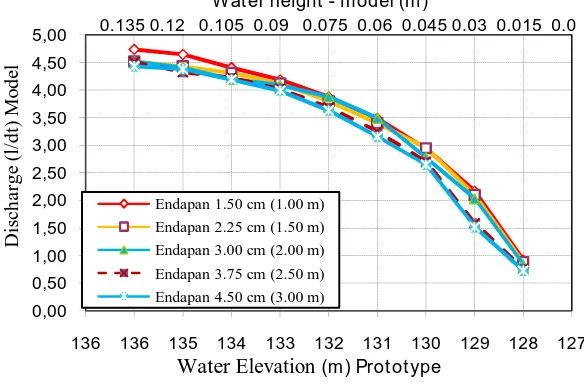
26 Figure. 4 Curve of Elevation-Discharge
Figure. 5 Curve of Elevation- L Erotion
Figure. 6 Curve of Elevation-Velocity
0,00 0,50 1,00 1,50 2,00 2,50 3,00 3,50 4,00 4,50 5,00
136 136 135 134 133 132 131 130 129 128 127
Endapan 1.50 cm (1.00 m) Endapan 2.25 cm (1.50 m) Endapan 3.00 cm (2.00 m) Endapan 3.75 cm (2.50 m) Endapan 4.50 cm (3.00 m)
D
is
ch
a
rge
(l
/dt
)
M
o
de
l
Water Elevation(m) Prot ot ype Wat er height - model (m)
0.135 0.12 0.105 0.09 0.075 0.06 0.045 0.03 0.015 0.0
0 2 4 6 8 10 12 14
136 136 135 134 133 132 131 130 129 128 127
L
C
o
m
E
ro
ti
o
n
(
c
m
)
m
o
d
e
l
Water Elevation (m) Prototype
Lk Endapan 1.50 cm (1.00 m) Lk Endapan 2.25 cm (1.50 m) Lk Endapan 3.00 cm (2.00 m) Lk Endapan 3.75 cm (2.50 m) Lk Endapan 4.50 cm (3.00 m)
Wat er height - model (m)
0.135 0.12 0.105 0.09 0.075 0.06 0.045 0.03 0.015 0.0
0 2 4 6 8 10 12
136 136 135 134 133 132 131 130 129 128 127
Endapan 1.50 cm (1.00 m) Endapan 2.25 cm (1.50 m) Endapan 3.00 cm (2.00 m) Endapan 3.75 cm (2.50 m) Endapan 4.50 cm (3.00 m)
V
e
lo
c
it
y
(c
m
/d
t)
Wat er Elevat ion (m ) Prot ot ype
Wat er height - model (m)
27 Figure. 7 Curve of Elevation - Concentration
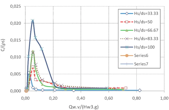
Figure 8 Relation C/(ρs) vs Qw .v/(Hw3.g) Each sediment thickness
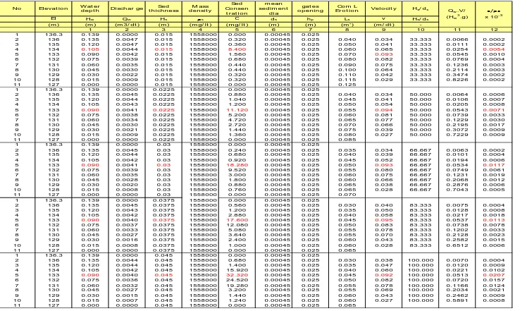
The result of parameter calculation in Table 8, can be
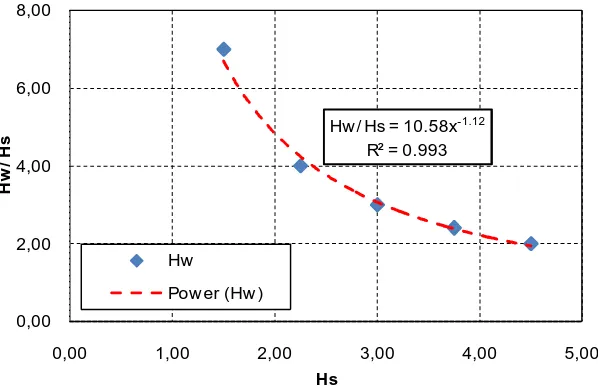
drawn as in figure 7. From figure 7 it shows that every sediment thickness Hs is gotten a value of C/(ρs) maximum. The value relation between C/(ρs) maximum and Qw .v/(Hw3.g) in every sediment thicknessis as in Tabel.7 below. If the graphic is made between the relation of Hw/Hs vs Hs at C maximum condition ( figure 8) it will be obtained the correlation between Hs dan Hw as:
Hw/Hs = 10.58 Hs-1.12, or : Hw = 10.58 Hs-0.12 with value of
R2=0.993 (look at figure 8). Thereby , it has very good correlation.
Table 7. Value of C/(ρs) maximum
5.39 1.00 1.50 10.50 7.00 7.13 1.50 2.25 9.00 4.00 11.73 2.00 3.00 9.00 3.00 11.30 2.50 3.75 9.00 2.40 20.74 3.00 4.50 9.00 2.00
0.025 0.054 0.053 0.053 0.051
C/(ρw)
M ax (106) Qw.V/ (Hw
3
.g) Hs Prototype (m)
Hs M odel (cm)
Hw M odel (cm)
28
Tabel 8. Calculation of Parameter C/(ρs) and Qw .v/(Hw3.g)
No El evat io n W at er
dep t h Di sch ar ge
Sed t h ichness
M ass d ensi t y
Sed Co nsen
t r at i on
m ean sedi m en t
di a
gat es o penin g
Co m L
Er o t io n Vel o ci t y Hs/ ds
El Hw Qw Hs ρs C ds hp Ls v Hs/ ds
(m ) (m ) (m 3/ dt ) (m ) (m g/ lt ) (m g/ lt ) (m ) (m ) (m ' ) (m / dt )
-1 2 3 4 5 6 7 8 9 10 11 12
1 136.3 0.139 0.0000 0.015 1558000 0.000 0.00045 0.025
2 136 0.135 0.0047 0.015 1558000 0.320 0.00045 0.025 0.040 0.034 33.333 0.0066 0.0002
3 135 0.120 0.0047 0.015 1558000 0.360 0.00045 0.025 0.050 0.041 33.333 0.0111 0.0002
4 134 0.105 0.0044 0.015 1558000 8.400 0.00045 0.025 0.060 0.065 33.333 0.0254 0.0054
5 133 0.090 0.0042 0.015 1558000 1.560 0.00045 0.025 0.070 0.093 33.333 0.0545 0.0010
6 132 0.075 0.0039 0.015 1558000 0.680 0.00045 0.025 0.080 0.082 33.333 0.0769 0.0004
7 131 0.060 0.0035 0.015 1558000 0.440 0.00045 0.025 0.090 0.075 33.333 0.1236 0.0003
8 130 0.045 0.0030 0.015 1558000 0.440 0.00045 0.025 0.100 0.064 33.333 0.2114 0.0003
9 129 0.030 0.0022 0.015 1558000 0.320 0.00045 0.025 0.110 0.042 33.333 0.3474 0.0002
10 128 0.015 0.0009 0.015 1558000 0.320 0.00045 0.025 0.115 0.029 33.333 0.8226 0.0002
11 127 0.000 0.0000 0.015 1558000 0.000 0.00045 0.025 0.125
1 136.3 0.139 0.0000 0.0225 1558000 0.000 0.00045 0.025
2 136 0.135 0.0045 0.0225 1558000 0.880 0.00045 0.025 0.040 0.034 50.000 0.0064 0.0006
3 135 0.120 0.0044 0.0225 1558000 1.040 0.00045 0.025 0.045 0.041 50.000 0.0106 0.0007
4 134 0.105 0.0043 0.0225 1558000 1.200 0.00045 0.025 0.050 0.054 50.000 0.0205 0.0008
5 133 0.090 0.0041 0.0225 1558000 11.120 0.00045 0.025 0.055 0.094 50.000 0.0543 0.0071
6 132 0.075 0.0038 0.0225 1558000 5.200 0.00045 0.025 0.060 0.081 50.000 0.0739 0.0033
7 131 0.060 0.0034 0.0225 1558000 4.720 0.00045 0.025 0.065 0.077 50.000 0.1229 0.0030
8 130 0.045 0.0030 0.0225 1558000 2.720 0.00045 0.025 0.070 0.066 50.000 0.2195 0.0017
9 129 0.030 0.0021 0.0225 1558000 1.440 0.00045 0.025 0.075 0.039 50.000 0.3072 0.0009
10 128 0.015 0.0009 0.0225 1558000 1.360 0.00045 0.025 0.080 0.027 50.000 0.7229 0.0009
11 127 0.000 0.0000 0.0225 1558000 0.000 0.00045 0.025 0.085
1 136.3 0.139 0.0000 0.03 1558000 0.000 0.00045 0.025
2 136 0.135 0.0045 0.03 1558000 0.240 0.00045 0.025 0.035 0.034 66.667 0.0063 0.0002
3 135 0.120 0.0044 0.03 1558000 0.680 0.00045 0.025 0.040 0.039 66.667 0.0101 0.0004
4 134 0.105 0.0042 0.03 1558000 0.920 0.00045 0.025 0.045 0.052 66.667 0.0194 0.0006
5 133 0.090 0.0041 0.03 1558000 18.280 0.00045 0.025 0.050 0.093 66.667 0.0534 0.0117
6 132 0.075 0.0039 0.03 1558000 9.520 0.00045 0.025 0.055 0.080 66.667 0.0749 0.0061
7 131 0.060 0.0035 0.03 1558000 3.000 0.00045 0.025 0.060 0.075 66.667 0.1231 0.0019
8 130 0.045 0.0028 0.03 1558000 1.800 0.00045 0.025 0.060 0.066 66.667 0.2068 0.0012
9 129 0.030 0.0020 0.03 1558000 0.880 0.00045 0.025 0.065 0.038 66.667 0.2876 0.0006
10 128 0.015 0.0008 0.03 1558000 0.760 0.00045 0.025 0.065 0.028 66.667 0.7043 0.0005
11 127 0.000 0.0000 0.03 1558000 0.000 0.00045 0.025 0.070
1 136.3 0.139 0.0000 0.0375 1558000 0.000 0.00045 0.025
2 136 0.135 0.0045 0.0375 1558000 0.560 0.00045 0.025 0.030 0.040 83.333 0.0075 0.0004
3 135 0.120 0.0043 0.0375 1558000 1.200 0.00045 0.025 0.035 0.050 83.333 0.0128 0.0008
4 134 0.105 0.0042 0.0375 1558000 2.880 0.00045 0.025 0.040 0.058 83.333 0.0217 0.0018
5 133 0.090 0.0040 0.0375 1558000 17.600 0.00045 0.025 0.045 0.095 83.333 0.0537 0.0113
6 132 0.075 0.0037 0.0375 1558000 12.080 0.00045 0.025 0.050 0.083 83.333 0.0738 0.0078
7 131 0.060 0.0033 0.0375 1558000 5.080 0.00045 0.025 0.055 0.078 83.333 0.1202 0.0033
8 130 0.045 0.0027 0.0375 1558000 3.640 0.00045 0.025 0.055 0.070 83.333 0.2128 0.0023
9 129 0.030 0.0016 0.0375 1558000 2.400 0.00045 0.025 0.060 0.043 83.333 0.2582 0.0015
10 128 0.015 0.0008 0.0375 1558000 1.000 0.00045 0.025 0.060 0.028 83.333 0.6512 0.0006
11 127 0.000 0.0000 0.0375 1558000 0.000 0.00045 0.025 0.065
1 136.3 0.139 0.0000 0.045 1558000 0.000 0.00045 0.025
2 136 0.135 0.0044 0.045 1558000 0.680 0.00045 0.025 0.030 0.038 100.000 0.0070 0.0004
3 135 0.120 0.0044 0.045 1558000 1.400 0.00045 0.025 0.035 0.047 100.000 0.0120 0.0009
4 134 0.105 0.0042 0.045 1558000 15.920 0.00045 0.025 0.040 0.060 100.000 0.0221 0.0102
5 133 0.090 0.0040 0.045 1558000 32.320 0.00045 0.025 0.045 0.092 100.000 0.0513 0.0207
6 132 0.075 0.0036 0.045 1558000 24.520 0.00045 0.025 0.050 0.082 100.000 0.0720 0.0157
7 131 0.060 0.0032 0.045 1558000 19.280 0.00045 0.025 0.055 0.078 100.000 0.1166 0.0124
8 130 0.045 0.0027 0.045 1558000 3.200 0.00045 0.025 0.055 0.069 100.000 0.2034 0.0021
9 129 0.030 0.0015 0.045 1558000 1.440 0.00045 0.025 0.060 0.043 100.000 0.2462 0.0009
10 128 0.015 0.0007 0.045 1558000 1.240 0.00045 0.025 0.060 0.027 100.000 0.5891 0.0008
11 127 0.000 0.0000 0.045 1558000 0.000 0.00045 0.025 0.065
Qw.V/
(Hw 3
.g)
c/ρs
29 Figure. 9 Correlation of Hw/Hs vs Hs
Statistical Analysis of the sediment concentration models
Generally, the multiple linear regression model stated that relation between the response variable of sediment concentration (C) with the predictor variables discharge (Qw), water depth (Hw), high sediment (Hs) and velocity (V) can be expressed by the equation:
i
e
V
Hs
Hw
Qw
C
i
i i i i 4 3 2
1
(
)
(
)
(
)
)
(
or can be written as:
With
0
ln(
)
and εi ~ NID(0,2
).Empirical result of regression model which was built based on data observation with the quantity of sample as much as N, is as follows:
1. Regression Significance Test ( F test )
To know about linear relation between response variable with predictor variables through F test. The details can be explained as follows:
a.Hypothesis formula :
0
:
1 2 3 40
H
0
:
1
ada
j
H
with j = 1,2,3,4b.Significance Level
5
%
c.Statistical Test)
1
/(
/
k
n
SSE
k
SSR
MSE
MSR
F
distributed F withfree degrees (k, n-k-1).
Testing Procedures
H
0:
j
0
is calculating1
/
/
0
k
n
SSE
k
SSR
F
then, compare with
F
F
tabel
α;k;nk1d. Refusal Criteria
H0 refused if F0=s Fhitung > Ftabel or H0 is refused if
p-value (sig.) < α=5%.
From Anova table if it is obtained that sig. < 0.05, it means that there is a significant linear relation between predictor variables discharge, water depth (In(Hw)), height of sediment (In(Hs)) and velocity (In(V)) with sediment concentration variable (In(C)) with contribution value of 76.2% (based on Adjusted R Square value).
2. Individual Parameter test ( t Test )
Individual test is used to test whether there is influence of each dependent variable towards linear regression model.
a. Hypothesis Formula :
0
:
0 j
H
0
:
1 j
H
with j = 1,2,3,4 b. Significance level
5
%
c. Statistical test :
jj
Se
t
ˆ
ˆ
distributed student-t with freedegrees (n-k-1);
with :
Se
ˆ
j
var
ˆ
jd. Refusal Criteria
Refused Ho if |thitung | >ttabel ( ttabel = t (1- /2,n-k-1)) If p-value (sig.) < α=5%.
Based on the value in coefficient table , the result of SPSS is obtained that all predictor variables of discharge (ln(Qw)), water depth (In(Hw)), height of sediment (In(Hs)) and velocity (In(V)) have a significant influence toward the response of sediment concentration ln C (p-value (sig) to parameters
1,
2,
3,
4 < 0.05), the model Hw / Hs = 10.58x-1.12R² = 0.993
0,00 2,00 4,00 6,00 8,00
0,00 1,00 2,00 3,00 4,00 5,00
H w / H s Hs Hw
30 doesn’t contain Constanta because = 0.
Thereby, the model can be estimated as:
ln = −3.515 ln( ) + 2.134 ln( ) + 0.983 ln( ) + 3.525 ln( )
Discussion
From Graphic relations between Water Surface Elevation and discharge (figure 4), it showed that the discharge for all variations of sediment thickness decreases slowly from elevation 136.00 to elevation 130.00 m, and decreases sharper starting from elevation 129.00 m. It is because in that elevation is a transition of flow behavior from flow with pressure to free flow.
Graphic relation between Water Surface Elevation and velocity (figure 6) looked rather similar. On the condition of high Water Surface Elevation between + 136 until 134m, flow velocity on the range of 150 cm upstream gate is varies. The lower the water surface, the higher the velocity, although the increase is not sharp. From water surface elevation of +134 decreasing to +133 m, Velocity raises sharper, and in elevation of +133 m, velocity reaches the maximum. If the water surface decreases again, the velocity decreases to ramps up to the elevation of +130.00 m , and then the velocity decreases until the end. The low velocity in still high water surface elevation is caused by the influence of puddle areas. From this experiment, it is showed that velocity is high, an average occurs in the range between elevation of +134 m - +130 m.
Graphic relation between Water surface elevation and Concentration (figure 7) shows that concentration values are vary, but they have the same pattern. On high water surface elevation, the concentration value is low, and if water surface elevation is decreased again, then the concentration will increase to certain value. If the water surface decreases again, the concentration start to lower/decrease. On this research, it is showed that generally, the higher the sediment thickness, the larger the value of sediment concentration in the same water surface position, especially between water surface elevation of +134 until +131 m. Meanwhile, on high of water surface elevation between +136 m and +135m, and low water surface elevation between +130 until +128 m, the difference of concentration is not significant. For sediment thickness of 1.50 cm, the maximum concentration is on elevation +134 m. For sediment thickness: 2.25; 3.00; 3.75; 4.50 cm, the maximum concentration is obtained on water surface elevation of +133 m.
The larger the sediment thickness showing that the position of water surface elevation which produces big concentration value is decreases, and the range is wider. On sediment thickness of 1,50 cm, the range of water surface elevation which produces high concentration is between +135 m – 133m. Sediment thickness of 2,25 cm, water surface elevation’s range which produces high concentration is between +134 m – 132 m. Sediment thickness of 3,00 cm and 3,75 cm, elevation’s range is between +134 m - +131 m, and for thickness of 4,50 cm,
elevation’s range which produces higher wider concentration is +135 m - +130 m. The pattern of the increase and decrease of concentration value corresponds with the pattern of the increase and decrease of velocity. This matter is reasonable, with low velocity will produce low scour concentration, and on high velocity will produce high scour concentration.
From dimensional analysis, it is obtained an equation from non-dimensional relation, so it will be discovered the relative roles of each parameter. The relation obtained is :
= .
. , and the correlation graphic is as in
figure 8. From the equation and picture, it is showed that parameter Hw is very dominant. C Value is a dependent parameter, greatly affected by Hw,g value, which is an independent parameter, and Qw and v dependent parameter. The graphic described that the value of parameter combination of a small .
. , will produce
small C, and if the value is bigger, C value will be bigger up to a certain point. When the value of .. is getting bigger, C Value will decrease. It can be expected that the value of C maximum is obtained on specific water surface elevation. If it is seen in the experiment data on Table 8, on the maximum points of is obtained the value of .
. , Hs and Hw are specific. Resume from value
of maximum and value .. , Hs and Hw is related as in Table 7 . From that data, it can be correlated between Hw/Hs vs Hs ( Figure 9) and the result:
Hw/Hs = 10.58 Hs-1.12, or Hw= 10.58 Hs-0.12 with determinant value R2 = 0.993 (strong correlation). Hw , is the same as the height of effective water surface (Hef)
Based on statistical analysis result and assumption testing (residual analysis): normality test, variants similarity, independent error, and multi-co linearity, then the best model which stated the relation between discharge predictor variables Qw, water surface Hw, sediment thickness Hs, velocity v, with concentration variable C is :
=
. . .
.
CONCLUSIONS AND SUGGESTIONS
Conclusions
1.Effective water surface on pressure flushing is the function of sediment thickness , that is :
Hef= 10.58 Hs-0.12
2.Application of pressure flushing with water surface above or below effective water surface, the result is less effective.
31 4.The big concentration in pressure flushing application
with water drawdown with gate opening of 2.50 cm is the function of Qw, Hs, Hw, and V , as follows :
=
. . .
.
Suggestions
This research is conducted with coal dust as the substitute for sand. There need to be more research with the same material but with variations of several diameters. On this research of discharge observations, velocity and concentration is conducted every water surface decreases 1.50 cm. There need to be a research for observations which are conducted on a denser interval of water surface lowering, for example every decrease of 0.75 cm (equivalent in prototype 0.50 m).
REFERENCES
[1]. Atkinson E., 1996, The Feasibility of Flushing Sediment from
Reservoir, TDR Project R 5839, Report OD 137, November 1996,
HR Wallingford,UK
[2]. Fan,J., and Jiang,R, 1980, On Methods For The Desiltation of
Reservoir, International Seminar of Expert on Reservoir
Desiltation, Tunis.
[3]. Meshkati, M.E., Dehghani A.A., Naser G., Emamgholizadeh,S., and Mosaedi, A., 2009. Evolution of Developing Flushing Cone
During The Pressurized Flushing in Reservoir Storage, World
Academic of Science, Engineering and Technology 58 2009
[4]. Montgomery, D.C and Peck, E, 1982. Introduction to Linear
Regression Analysis. John Weley & Sons, Singapore.
[5]. Morris G.L and Fan J, 1998, Reservoir Sedimentation Handbook
Design and Management of Dam,Reservoir, and Watersheds for Sustainable Use, McGrow-Hill Companies,Inc., New York.
[6]. Nippon Koei Co. LTD., 2009, Detail Design of Structural Counter
Measures for Sedimentation On Wonogiri Reservoir, Volume I :
Design Report, BBWS Bengawan Solo
[7]. Scheuerlein Helmut,1993, Estimation of Flushing Efficiency in
Silted Reservoir, Proceeding of The International Conference on
Hydro-Science an –Engineering, Wasington,DC,June 7-11,1993 [8]. Sinaro, R., Kasiro, I., Brotodiharjo, A., Widyarso, T., 2007.
Menyimak Bendungan di Indonesia (1910-2006),
Indocamp,Jakarta.
[9]. Strand, R.I. and Pemberton, E.L,. 1987. Reservoir Sedimentation. In Design Small Dams, US. Bereau of Reclamation, Denver [10].Xia,Z. and Zhang,Q, 1980, Reservoir Sedimentation, International
Symposium on River Sdementation, P.D(I) 1-13, Chinese Society oh Hydraulic Engineering, Bejing, People’s Republic of China.
[11].Yang Chih Ted, 1996 Sediment Transport Theory and Practice, McGraw-Hill,Singapore.
[12].Yoon, Y. N,. 1992. The State and The Perspective of The Direct
Sediment Removal Method From Reservoir. International Journal