Parameter Estimation in LNSV Models:
Griddy Gibbs versus Metropolis-Hastings
Abstract
This paper compares performances of two MCMC samplers, Griddy-Gibbs (GG) and Metropolis-Hastings (MH) samplers, to estimate parameters and latent variables in the four log-normal stochastic volatility (LNSV) models: (1) LNSVn (standard), (2) LNSVt (with fat-tails), (3) LNSVL (with correlated errors), (4) LNSVLt (with fat-tails and correlated errors). To illustrate the comparison of two samplers, we apply the mod-els and samplers to both simulated and real data sets. The stock indices we examine are TOPIX and three stocks of the TOPIX Core 30: Hitachi Ltd., Nissan Motor Co. Ltd. and Panasonic Corp.
Keywords: Log-normal stochastic volatility, Bayesian inference, single-move Markov Chain Monte Carlo, Griddy Gibbs, Metropolis-Hastings, TOPIX.
1 Introduction
Amongst modeling of financial time series, the stochastic volatility (SV) model is re-cognized as one of the most important class as it has the ability to capture the commonly observed change in variance of the observed stock index or exchange rate over time. A popular and most widely used SV model is the log-normal (LN) SV model, which was first introduced by Taylor (1982). In his discrete time model, volatility process is modeled as a first-order autoregression for the log-squared volatility. The LNSV model provides a more realistic and adequate than the ARCH-type models (see, for example, Ghysels et al. (1996)) and the GARCH-type models (see, for example, Kim et al. (1998), Yu (2002) and Carnero et al. (2001)).
Unfortunately, it is not possible to take random draws directly from the posterior for some unknown parameters in SV models. An approach has become very attractive is the Bayesian approach, which was first proposed by Shephard (1993) and Jacquier et al. (1994). Inference in this approach often requires advanced Bayesian computation, and here we focus on Markov Chain Monte Carlo (MCMC) procedure to perform posterior sampling and statistical inference. MCMC permits to obtain the conditional posterior distributions of the parameters by simulation rather than analytical methods. To summarize posterior
∗The email addresses of the authors are, respectively, [email protected] and
[email protected]. The first author is a PhD candidate. The first author also wishes to thank Shuichi Nagata for some Matlab codes and helpful discussions.
2
Didit B. Nugroho 1,2 and Takayuki Morimoto
Department of Mathematics, Satya Wacana Christian University Department of Mathematical Sciences, Kwansei Gakuin University
June 25, 2012
2
distributions, it is necessary to have algorithms that are well-suited to updating random samples (e.g. Gibbs sampling, Metropolis-Hastings and Griddy-Gibbs sampler).
Comparison of Metropolis-Hastings (MH) algorithm and Griddy-Gibbs (GG) sampler has already been discussed in Bauwens and Lubrano (1998) for an asymmetric StudentGARCH model. They show that GG sampler is feasible and competitive compared with MH sampler. In this paper we compare the performance between the use of the GG sampler and the MH sampler to estimate four LNSV models fitted to both simulated and real data sets. The real data we analysis includes the high frequency data sets for computing realized volatility (RV) and daily returns of TOPIX and three stocks of the TOPIX Core 30, which are Hitachi Ltd., Nissan Motor Co. Ltd. and Panasonic Corp., from January 5, 2004 until December 30, 2011. RV is used as a proxy to evaluate the daily estimated volatility performances. It was showed by Anderson et al. (2003) that the daily RV obtained from the intra-day high frequency data set is an consistent and robust estimator of the ”true” volatility.
The rest of this paper is organized as follows. The model specification is discussed in Section 2. Section 3 presents the description of the Bayesian MCMC method, conditional posteriors and sampling algorithms. In Section 4, we apply the model and the samplers to the daily returns on three stocks to obtain volatilities and values of model parameters. Finally, Section 5 gives some concluding remarks.
2 MCMC Methods
The Gibbs sampling algorithm (Geman and Geman. (1984)) uses a sequence of draws from conditional distributions to characterize the joint target distribution. Suppose that our parameter vectorθhas two components, making our target distributionf(θ1, θ2|y). To use the Gibbs sampler, one begins by choosing starting values θ2(0) (starting values are usually chosen near the posterior mode or the maximum likelihood estimates). One then repeats, fori= 1, ..., N iterations (making sure to store the sequence of draws at each iteration):
Step 1: Sample θ1(i+1) frompθ1|θ(2i), y
.
Step 2: Sample θ2(i+1) frompθ2|θ(1i+1), y.
Metropolis-Hastings algorithm is first introduced by Metropolis et al. (1953) and general-ized by Hastings (1970). The algorithm has many applications beyond Bayesian statistics; it is commonly used for all sorts of numerical integration and optimization. (It is also the case that the Gibbs sampling algorithm is a special case of the Metropolis-Hastings algorithm.) To simulate from our target distribution p(θ|y), we again start with sensible starting values: θ(0). For each iteration of the simulationi= 1, ..., N, we draw a proposalθ∗ from a known proposal distributionp θ∗|θ(i). Unlike the Gibbs sampling algorithm, when each move is automatically accepted, one accepts the proposal distribution probabilistically, sometimes moving to a value with a higher density value, sometimes moving to one with a lower density value.
Unlike the MH sampler, in the GG sampler we do not need to find an efficient proposal distribution.
3 Accuracy
Without being able to plot the target distribution, which in most applications is of high dimension, it would be difficult, if not impossible, to assess whether the chain is sampling from the target distribution. An important part of any Bayesian analysis is assessing the convergence of the simulation results. Indeed, no Monte Carlo estimates of posterior density summaries can be trusted unless the chain has reached its steady state.
4 LNSV Model with Fat-tails and Correlated Errors
We consider the lognormal stochastic volatility (LNSV) model given by
Rt = e
1
2htωt, ωt=λ−
1 2
t ǫt, ǫtiid∼ N(0,1), t= 1, ..., T, (1)
ht+1 = α+φ(ht−α) +τ ηt+1, ηt+1iid∼ N(0,1), t= 1, ..., T−1, (2) λt ∼ p(λt|ν)
corr(ǫt, ηt+1) = ρ
where ht = lnσt2, for the unobservable volatility σt of asset on day t, Rt is the asset
return on day t from which the mean and autocorrelations are removed, 0 ≤ φ < 1, h1 ∼ N α, τ2/ 1−φ2, and N(·,·) represents the normal distribution. In this model, ν captures the fat-tailness and ρcaptures the leverage effect, which refers to the asymmet-ric behavior that return movements are negatively correlated with volatility. As pointed out in Yu (2005), specification ofcorr(ǫt, ηt+1) =ρ implies that the above model is a mar-tingale difference sequence and clear to interpret the leverage effect instead of assuming corr(ǫt, ηt) =ρ in Jacquier et al. (2004).
The above model has a parameter vector (ν, α, φ, τ2, ρ) and two latent stochastic pro-cesses denoted, respectively, by h = (h1, h2, ..., hT) and λ = (λ1, λ2, ..., λT), which are to
be estimated simultaneously using simulation methods which will be discussed in the next section. Here, the value of φ measures the autocorrelation present in the logged squared volatility. Thusφ can be interpreted as the persistence in the volatility, the constant scal-ing factor exp 12α as the modal instantaneous volatility, and τ is the volatility of the log-volatility (cf. Kim et al. (1998)). It is common to assume that 0≤φ <1 because the volatility is positively autocorrelated in most financial time series. Next,λtis a scale factor,
p(λt|ν) is the mixing density. We assume that λt is distributed i.i.d gamma, or that νλt
follows a χ2 distribution with 3 ≤ ν ≤ 40 degrees of freedom, as discussed by Watanabe and Asai (2001) and Jacquier et al. (2004). This assumption implies that the marginal distribution of λ−
1 2
t ǫt is Student-t withν degrees of freedom.
As in the previous literature (see, for example Zhang and King (2003, 2008), Jacquier et al. (2004) and Yu (2005)), it is convenient to write
ηt+1=ρǫt+ p
1−ρ2w
t+1, (3) fort= 1,2, ..., T−1, wherewt+1 is iidN(0,1) and corr(ǫt, wt+1) = 0. Transformation (3) shows that var(ηt+1) = 1 and corr(ηt+1, ǫt) = ρ which satisfies the above LNSV model
specification. Substituting (3) into (2), we obtain
ht+1=α+φ(ht−α) +ρτ e−
1 2htλ
1 2
tRt+ p
1−ρ2τ w
t+1.
It is evident that a unit increase in stock return at time tresults in aρτ σt−1λ
1 2
t unit change
a unit fall in stock return at this period will result in exp
ρτ σt−1λ
1 2
t
unit increase in the
variance at timet+ 1.1
Following Jacquier et al. (2004), and has been applied more recently by Yu (2005) and Zhang and King (2003, 2008), we re-parameterizedρandτ toϕ=ρτ andψ2 = 1−ρ2τ2, respectively, and obtain
Rt = e
1 2htλ−
1 2
t ǫt, ǫtiid∼ N(0,1), t= 1, ..., T, (4)
ht+1 = α+φ(ht−α) +ϕe−
1 2htλ
1 2
tRt+ψwt+1, wt+1iid∼ N(0,1), t= 1, ..., T−1,(5) where
h1∼ N α, ψ2/ 1−φ2 and ht|ht−1 ∼ N
α+φ(ht−1−α) +ϕe−
1 2ht−1λ
1 2
t−1Rt−1, ψ2
(6) for t = 2, ..., T. We now have a new parameter vector denoted by θ = (ν, α, φ, ϕ, ψ2).
Because ǫt and wt+1 are uncorrelated, we can now easily obtain the joint posterior ofh,λ and θ conditional on observations R, whereR= (R1, R2, ..., RT).
5 Prior Specification
Following standard practice, we assume that our model is completed by priors for the unknown structural parameters as follows:
λt∼ G(12ν,12ν), ν ∼ G(aν, bν), (7)
φ∼ B(A, B), ψ2∼ IG(a, b), α|ψ2 ∼ N α0, ψ2/p0, ϕ|ψ2 ∼ N ϕ0, ψ2/q0, (8)
whereB(·,·),IG(·,·) andG(·,·) represent the beta, inverse gamma and gamma distributions, respectively. For parameter ν, the following alternative priors were used in the previous literature: exponential by Geweke (1993), Watanabe and Asai (2001), uniform discrete on the interval [3,40] by Jacquier et al. (2004), Gaussian by Zhang and King (2008) and gamma on the interval (2,40] by Abanto-Valle et al. (2010). These priors are chosen to prevent ν from getting too large during MCMC iterations, because the update of ν has a negligible effect when ν is already large.
6 Bayesian Approach
In order to implement Gibbs sampling, all of the fully conditional posterior distributions (one for each component ofθ) need to be derived from the joint posterior distribution. The conditional posterior distribution is derived from the joint posterior distribution by picking out the parts that involve the unknown parameter in question.
Denote θ−ν be the parameter vector after removing ν. By using Bayes’ theorem, the
joint posterior distribution of parameters and latent unobservable variables conditional on the returns is
p(λ,h,θ|R) =p(R|h,λ)×p(λ|ν)×p(h|θ−ν)×p(θ), (9)
1
where
which are obtained from the likelihood function of R, the conditional and unconditional functions of h and the prior distributions in (7) and (8). A Gibbs sampler approach then estimates the parameters and latent variables by drawing random samples from the following conditional posterior distributions:
into the lower bound. In this case, the conditional posterior forλis obtained from the joint
The conditional posterior forλ is
shape and inverse scale parameters being defined, respectively, by
Aλt =
The above conditional posterior is only standard for t=T, and hence we sample directly λ1 from Gamma distribution and sample λt, for t = 1, ..., T −1, by using Griddy Gibbs
and Metropolis-Hastings. Because the fG distribution does not depend on λt, using the
Independence Chain (IC) MH sampling method introduced by Tierney (1994), we sample a proposal λ∗t ∼ G(Aλt, Bλt) and accept it with probability min{1, g1(λ
∗
t)/g1(λt)}.
The probability density function (PDF) of the standardized student-t distribution with degrees of freedomν >2 is given by
f(ωt) =
So the conditional posterior forν is
p(ν|h,R) =p(ν)f(ωt)∝νaν−1e−bνν
A problem arises here in that the above posterior is not standard, and hence we sample ν using Griddy Gibbs sampler and Metropolis-Hastings algorithm.
To sampleνby Hastings algorithm, we use the Independence Chain Metropolis-Hastings (IC-MH) sampling method, in which the proposal forν isν∗ ∼ N[3,40] µν, s2ν
and the acceptance probability is min{1, p(ν∗)/p(ν)}. The meanµν and variances2ν are
In this following, we write the above log posterior asℓ(ν) since after the data are observed,ν is only random quantity. We find the the posterior mode ˆν ofℓ(ν), meaning that ℓ′(ˆν) = 0, by numerical optimization, and then we take µν = ˆν and sν2 = −1/ℓ′′(ˆν). A very simple
and robust method for finding the mode ˆν is provided by bisection method,
ˆ
To see this, we use the result of Abramowitz and Stegun (1972) (see Eq. 6.1.38), in which the ln Γ(ν/2) is approximated by
ln Γ(x) = ln(2π)
Thus, withaν >1, the first term is always negative, and the second term is always positive.
Therefore, following Watanabe and Asai (2001) we set s2
ν =−1/Dν(ˆν) where
Dν(ˆν) = min
ℓ′′(ˆν),−0.0001 .
We should note that ℓ′′(ˆν) is always negative in our empirical analysis.
Given the conditional posterior for w, we propose the following Griddy Gibbs sampler procedure:
1. Denote the equally spaced grid of values for w, say,w1≤w2 ≤ · · · ≤wm.
2. Compute the value ofw’s posterior at each of the grid points and denote the resultant vector by p(w) = (p(w1), . . . , p(wm)).
3. Normalize p(w) and denote the resultant vector by p∗(w) = (p∗(w1), . . . , p∗(wm)).
4. Compute the empirical cumulative distribution function ofw, Φ(w).
5. Generateu∼U(0,Φ(wm)) and invert Φ(w) by linear interpolation to obtain a random
sample ofw.
7.2 Sampling α
For sampling α based on the joint posterior (9), we found that the logarithm of the conditional posterior forα is
wherezt=ht−φht−1−ϕe−
Based on the joint posterior (9), we found that the logarithm of the conditional posterior forϕis
and
ψ2 are sampled, respectively, from their conditional posteriors, we can calculate τ2 and ρ through τ2 =ϕ2+ψ2 and ρ= ϕ
τ.
7.5 Sampling φ
Based on the joint posterior (9), the log of the conditional posterior for φis given by
lnp(φ|h,λ,θ−ν,R) ∝ lnp(φ) + ln 1−φ
Hence the conditional posterior forφcan be expressed as
p φ|h, α, ϕ, ψ2∝fN φ|µφ, s2φ mean µ and variance s2. The above conditional posterior is not standard, and hence we draw φby Griddy Gibbs sampler and Metropolis-Hastings algorithm.
We note that a fN
φ|µφ, s2φ
distribution does not depend on φ. Therefore, using the
IC-MH sampling method, we sample a proposal φ∗ ∼ N[0,1)
Denoteh−tbe the latent stochastic vector after removinght. Based on the joint posterior
where wt = ht−Rtλ
1 2
t, for t = 1, ..., T −1. In order to sample h, we use the Griddy
Gibbs sampler and the random walk Metropolis-Hastings algorithm, in which the proposal density is the standar normal and the acceptance probability is computed through (12). In this case, the proposal value h∗t at (i+ 1)th iteration is generated according to the process
h∗t =h(ti)+ǫ(ti+1), whereǫ(ti+1)∼ N0, ψ2(i+1).
7.7 Single Move MCMC
Since the conditional posteriors of ν,φ and h do not have closed form, we first sample the latent variableλand parametersα,ϕandψ2. The Gibbs sampling scheme is described
as follows. Choose arbitrary starting values θ(0),λ(0) andh(0), and leti= 0.
1. Sampleλ(i+1) fromp λ|ν(i),h(i),R.
2. Sampleν(i+1) from p ν|h(i),R.
3. Sampleα(i+1) from pα|λ(i+1),h(i), φ(i), ϕ(i), ψ2(i),R.
4. Sampleϕ(i+1) frompϕ|λ(i+1), α(i+1),h(i), φ(i), ψ2(i),R.
5. Sample ψ2(i+1) from pψ2|λ(i+1), α(i+1), ϕ(i+1),h(i), φ(i),R.
6. Sampleφ(i+1) frompφ|λ(i+1), α(i+1), ϕ(i+1), ψ2(i+1),h(i),R.
7. Sampleh(i+1) from ph|λ(i+1),θ(−i+1)ν ,R.
8. Seti=i+ 1 and go to step 1 until convergence is achieved.
8 Comparison of MCMC Methods
8.1 Simulated Data
8.2 Stock Market Data
8.2.1 Data Description
In this section we apply the methods and LNSV models used previously to the series of daily closing prices {St} of the TOPIX and three stocks of the TOPIX Core 30, which
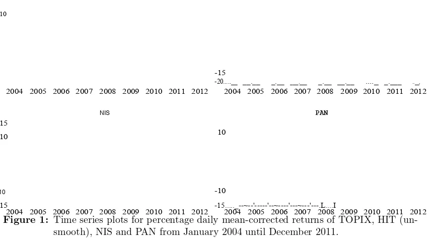
are Hitachi Ltd. (HIT), Nissan Motor Co. Ltd. (NIS) and Panasonic Corp. (PAN), from January 5, 2004 until December 30, 2011, for a total of 1960 observations. The series of return are daily percentage mean-corrected returns,Rt, given by the transformation
Rt= 100× ln
St
St−1 − 1 T
T X
i=1 ln Si
Si−1 !
Figure 1: Time series plots for percentage daily mean-corrected returns of TOPIX, HIT (un-smooth), NIS and PAN from January 2004 until December 2011.
Table 1 reports summary statistics for the returns data, and Figure 1 displays the series of returns data. As usual, the kurtosis of the returns is significantly above three, indi-cating leptokurtic return distributions. The Ljung-Box (LB) test statistics indicate that the returns for TOPIX, NIS and PAN stock price indices are serially uncorrelated, while the returns for HIT index is serially correlated at the 5% level. One simple way to adjust these autocorrelated returns is to unsmooth the return series such that the adjusted returns display no serial correlation. The procedure is given as follows (see De Souza and Gokcan (2004)):
R∗t = Rt−ρkRt−k 1−ρk
where ρk is the kth-order autocorrelation of the autocorrelated return seriesRt, andRt−k
is the k-period lagged return.
Table 1: Descriptive statistics of the daily returns for TOPIX and TOPIX Core 30.
Statistics TOPIX HIT NIS PAN
Raw Data Raw data Unsmooth Raw data Raw data
Sample size 1961 1961 1959 1961 1961
Mean 0.000 0.000 −0.001 0.000 0.000 Standard deviation 1.479 2.195 2.065 2.360 2.113 Kurtosis 11.245 11.390 11.178 8.669 8.353 LB(8) 9.026 18.227 10.295 15.136 12.682 p-value LB(8) 34.00% 1.96% 24.49% 5.65% 12.33%
Autocorrelation no yes no no no
NOTE: The lag lengths= 8 for the LB(s) statistic is selected based on the choice ofs≈ln(1961) (see Tsay (2010)).
10
HIT
-15
-20..._ _ __. __ _._ _ ___. __ _._ _ __. __ ...._ _ _._ __ ..__, 2004 2005 2006 2007 2008 2009 2010 2011 2012 2004 2005 2006 2007 2008 2009 2010 2011 2012
NIS
15
10
-10
PAN
10
-15 -15..._--~--'---'--~----'---~---'---.L....I
8.2.2 Estimation Results
In our analysis, we compare two proposed MCMC methods for the following four candi-date LNSV models:
1. Model SVn: the LNSV model without both fat-tails and correlated errors. The error in return is assumed to follow normal distribution (λt = 1 for all t), and there is no
correlation between errors in return and volatility (ρ= 0).
2. Model SVt: the LNSV model with fat-tails. The error in return is assumed to Student-t distribution with unknown degrees of freedom, and there is no correlation between errors in return and volatility.
3. Model SVL: the LNSV model with correlated errors. The error in return is assumed to follow normal distribution, and there is a correlation between errors in return and volatility (ρ6= 0).
4. Model SVLt: the LNSV model with fat-tails and correlated errors. The error in return is assumed to Student-tdistribution with unknown degrees of freedom, and there is a correlation between errors in return and volatility.
The hyperparameters in (7) and (8) required in the joint prior distribution were set to aν = 12,bν = 0.8,A= 30,B = 1.5,a= 1,b= 0.005,α0 = 0,p0 = 0.2,ϕ0= 0 andq0= 0.5. For initial parameter values and log-volatilities, respectively, we setθ(0) = (20,1,0.9,0.1,0.1) and h(0)t = 2 lnRV. In particular, Griddy Gibbs samples of ν, φ and ht are, respectively,
drawn using 100, 200 and 400 equally spaced points. The possible range of ht for the ith
Gibbs iteration is [h(ti−1) −1, h(ti−1) + 1]. In all cases, we simulated the ht’s in a
single-move fashion. All the calculations were performed running stand alone code developed by the authors using MATLAB version 7.8.0(R2009a) on a AMD Phenom(tm) II X6 1035T Processor 2.60GHz.
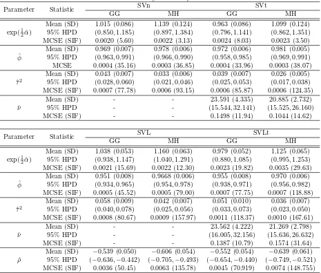
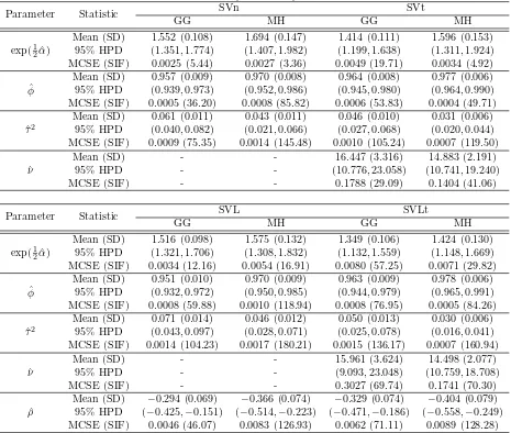
For all the models and methods, we ran the MCMC simulation for 15000 iteration but discarded the first 5000 draws. With the resulting N = 10000 values, we calculated the posterior means, standard deviations (SD), the 95% credible interval, the Monte Carlo standard error (MCSE) and the simulation inefficiency factors (SIF). Table 2, 4, 6 and 8 summarize these results. According to both MCSE and SIF, the two proposed sampling algorithms have been mixing quite good. The 95% credible intervals are calculated using a highest posterior density (HPD) proposed by Chen and Shao (1999). The MCSE is estimated by σbf/
√
N (see Roberts (1996)), where bσf2 id defined as the variance of the posterior mean from correlated draws. Here, the number of batches was 50 and there were 200 draws in each batch. The SIF can be interpreted as the number of successive iterations needed to obtain near independent samples and is calculated by bσf2/eσf2, where eσf is the
standard deviation of the posterior mean.
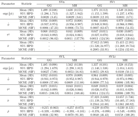
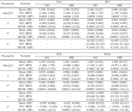
of shock to volatility, HL = ln(0.5)/ln( ˆφ) (see Hall (2005)). Third, the posterior means for the conditional variance of volatility, ˆτ2, are smaller by the MH sampler than those by the GG sampler for all cases, indicating that MH sampler exhibits a lower vari-ability of volatility. The lowest posterior mean is for SVLt model in MH sampler except for TOPIX, and the highest one is for SVL model in GG sampler. Fourth, the posterior means of the degrees of freedom, ν, in SV models with fat-tails are between 13 (for the Hitachi stock in the SVLt model by MH sampler) and 24 (for the TOPIX in the SVt by GG sampler), indicating that the normal conditional distribution would be strongly rejected by the data. In all cases, GG sampler exhibits the higher posterior means of the degrees of freedom of the Student-t distribution. Fifth, the posterior means of the leverage effect parameter, ρ, in all cases of SV models with correlated errors are in the negative interval, where posterior means in GG sampler suggest that some though weakerevidence of negative correlation between returns and volatility process.
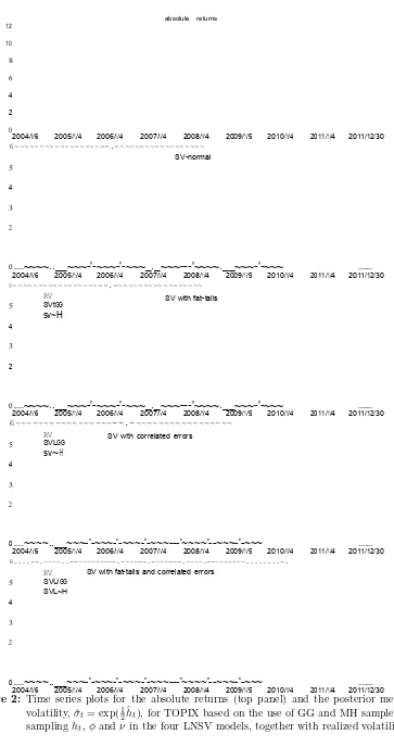
To evaluate the daily estimated volatility performances, the standard realized volatility (RV) is used as a proxy. It was showed by Anderson et al. (2003) that the daily RV obtained from the intra-day high frequency data set is an consistent and robust estimator of the ”true” volatility as long as there are no jumps. The percentage RV is defined by
RVt= 100× r
XNt
k=2[p(t, k)−p(t, k−1)] 2,
where Nt is the number of observations in day t and p(t, k) denotes the log-price at the
k’th observation in day t. To measure the closeness between the estimated volatilities and RV, six loss functions are used, namely, root mean-squared error (RMSE) for volatility and variance, mean absolute error (MAE) for volatility and variance, logarithmic loss (LL) and Gaussian quasi-maximum likelihood function (GMLE), as discussed by Bollerslev et al. (1994) and Lopez (2001).
Table 3, 5, 7 and 9 present the value and ranking (indicated by subscripts) of all four SV models and two samplers under the six statistical loss functions. An interesting result is thatfor the TOPIX series the GG sampler provides themost accurateestimates against the MH sampler in each model. In fact, of the eight cases the four best estimates are performed by the GG sampler, where the best performance is for SVLt model. For Hitachi, excluding GMLE loss function, the best estimate is provided by MH sampler, where five loss functions indicate that the SVL model provides the most accurate estimation. Excluding GMLE loss function, MH sampler for SVLt model is the best sampler to estimate volatility of Nissan indicated by five loss functons. The results for Panasonic series indicatesno clear pattern.
the posterior means of volatilities from the MH sampler exhibit smoother movements than those from the GG sampler. The figure is also nicely illustrated that RV and the estimated volatility closely mimic the movements of|Rt|plotted in the top panel supporting the idea
of using mean-corrected returns as proxies forht.
9 Conclusion
The results, based on daily observations from all four stocks using four LNSV models, reveal that volatility by MH sampler in all cases is more persistent and less variable than those by GG sampler. In the case of LNSV models with a fat-tails component, the degrees of freedom shows that the student-tdistribution by MH sampler appears flatters with heavier tails. In case the LNSV models with correlated errors, the posterior mean of leverage effect parameter involving the use of MH sampler show a stronger evidence of negative asymmetric returns-volatility relation. After comparing the estimation performance of all cases, where standard daily RV is used as a proxy, it was found that the GG sampler is superior according to all six loss functions for TOPIX in the LNSVLt model, while the MH sampler is superior according to five loss functions for Hitachi in the LNSVL model and for Nissan in the LNSVLt model and three loss functions for Panasonic in the LNSVt model. Furthermore, GMLE (Gaussian quasi-maximum likelihood function) loss function is only minimized on all stocks in the same model and sampler: LNSVLt model by GG sampler.
References
Abanto-Valle, C. A., Bandyopadhyay, D., Lachos, V. H., & Enriquez, I. (2010). Robust Bayesian analysis of heavy-tailed stochastic volatility models using scale mixtures of normal distributions. Computational Statistics and Data Analysis, 54(12), 2883– 2898.
Abramowitz, M., & Stegun, N. (Eds.). (1972). Handbook of mathematical functions with
formulas, graphs, and mathematical tables. Dover Publications Inc.
Albert, J. (2009). Bayesian computation with R (2nd ed.). Springer.
Anderson, T. G., Bollerslev, T., Diebold, F. X., & Labys, P. (2003). Modeling and fore-casting realized volatility. Econometrica,71, 529–626.
Bauwens, L., & Lubrano, M. (1998). Bayesian inference on GARCH models using the Gibbs sampler. The Econometrics Journal,1, 23–46.
Bollerslev, T., Engle, R. F., & Nelson, D. B. (1994). ARCH Models. In R. Engle & D. McFadden (Eds.), The Handbook of Econometrics (pp. 2959–3038). Amsterdam: North-Holland.
Carnero, M. A., Pea, D., & Ruiz, E. (2001). Is stochastic volatility more flexible than
GARCH? Working Paper 01-08, Universidad Carlos III de Madrid. Available from
e-archivo.uc3m.es/bitstream/10016/152/1/w
Chen, M. H., & Shao, Q. M. (1999). Monte Carlo estimation of Bayesian credible and HPD intervals. Journal of Computational and Graphical Statistics,8, 69–92.
De Souza, C., & Gokcan, S. (2004). Hedge fund volatility: It’s not what you think it is.
AIMA Journal.
Geman, S., & Geman., D. (1984). Stochastic relaxation, Gibbs distribution and Bayesian restoration of images. IEE Transactions on Pattern Analysis and Machine
Intelli-gence,6, 721–741.
Geweke, J. (1993). Bayesian treatment of the independent student-tlinear model. Journal
Ghysels, E., Harvey, A. C., & Renault, E. (1996). Stochastic volatility. In G. Maddala & C. Rao (Eds.), Handbook of Statistics: Statistical Methods in Finance (pp. 119–191). Amsterdam: Elsevier Science.
Hall, A. R. (2005). Generalized method of moments. Oxford University Press.
Hastings, W. K. (1970). Monte Carlo sampling methods using Markov chains and their applications. Biometrika,57(1), 97–109.
Jacquier, E., Polson, N. G., & Rossi, P. E. (1994). Bayesian analysis of stochastic volatility models. In N. Shephard (Ed.),Stochastic Volatility: Selected Readings (pp. 247–282). Oxford University Press, New York.
Jacquier, E., Polson, N. G., & Rossi, P. E. (2004). Bayesian analysis of stochastic volatility models with fat-tails and correlated errors. Journal of Econometrics, 122(1), 185– 212.
Kim, S., Shephard, N., & Chib, S. (1998). Stochastic volatility: likelihood inference and comparison with ARCH models. In N. Shephard (Ed.), Stochastic volatility: selected
readings. Oxford University Press.
Lopez, J. A. (2001). Evaluation of predictive accuracy of volatility models. Journal of
Forecasting,20(1), 87–109.
Metropolis, N., Rosenbluth, A. W., Marshall, N. R., Teller, A. H., & Teller, E. (1953). Equations of state calculations by fast computing machines. Journal of Chemical
Physics,21(6), 1087–1091.
Roberts, G. O. (1996). Markov chain concepts related to sampling algorithms. In R. S. Gilks W.R. & D. Spiegelhalter (Eds.),Markov Chain Monte Carlo in Practice (pp. 45–57). Chapman & Hall, London.
Sel¸cuk, F. (2008). Asymmetric stochastic volatility in emerging stock markets. Applied
Financial Economics,15(12), 867–874.
Shephard, N. (1993). Fitting non-linear time series models, with applications to stochastic variance models. Journal of Applied Econometrics,8, 135–152.
Taylor, S. J. (1982). Financial returns modelled by the product of two stochastic processes— a study of the daily sugar prices 1961–75. In N. Shephard (Ed.),Stochastic Volatility:
Selected Readings (pp. 60–82). Oxford University Press, New York.
Tierney, L. (1994). Markov chain for exploring posterior distributions. Annals of Statistics, 22(4), 1701–1762.
Watanabe, T., & Asai, M. (2001).Stochastic volatility models with heavy-tailed distributions:
a Bayesian analysis. In Bank of Japan, IMES Discussion Paper Series No. 2001-E-17.
Yu, J. (2002). Forecasting volatility in the New Zealand stock market. Applied Financial
Economics,12, 193–202.
Yu, J. (2005). On leverage in a stochastic volatility model. Journal of Econometrics, 127(2), 165–178.
Zhang, X., & King, M. L. (2003). Estimation of asymmetric Box-Cox stochastic volatility
models using MCMC simulation.Working Paper 10/03, Monash University. Available
from http://www.buseco.monash.edu.au/ebs/pubs/wpapers/2003/
Table 2: Posterior analysis for daily TOPIX.
Parameter Statistic SVn SVt
GG MH GG MH
exp(1 2αˆ)
Mean (SD) 1.015 (0.086) 1.139 (0.124) 0.963 (0.086) 1.099 (0.124) 95% HPD (0.850,1.185) (0.897,1.384) (0.796,1.141) (0.862,1.351) MCSE (SIF) 0.0020 (5.60) 0.0022 (3.13) 0.0024 (8.03) 0.0023 (3.50) ˆ
φ
Mean (SD) 0.969 (0.007) 0.978 (0.006) 0.972 (0.006) 0.981 (0.005) 95% HPD (0.963,0.991) (0.966,0.990) (0.958,0.985) (0.969,0.991) MCSE 0.0004 (35.16) 0.0003 (36.85) 0.0004 (33.96) 0.0003 (38.07) ˆ
τ2
Mean (SD) 0.043 (0.007) 0.033 (0.006) 0.039 (0.007) 0.026 (0.005) 95% HPD (0.028,0.060) (0.021,0.046) (0.025,0.053) (0.017,0.038) MCSE (SIF) 0.0007 (77.78) 0.0006 (93.15) 0.0006 (85.87) 0.0006 (124.35) ˆ
ν
Mean (SD) - - 23.591 (4.335) 20.885 (2.732) 95% HPD - - (15.544,32.141) (15.525,26.160) MCSE (SIF) - - 0.1498 (11.94) 0.1044 (14.62)
Parameter Statistic SVL SVLt
GG MH GG MH
exp(1 2αˆ)
Mean (SD) 1.038 (0.053) 1.160 (0.063) 0.979 (0.052) 1.125 (0.065) 95% HPD (0.938,1.147) (1.040,1.291) (0.880,1.085) (0.995,1.253) MCSE (SIF) 0.0021 (15.69) 0.0022 (12.30) 0.0023 (19.82) 0.0035 (29.63) ˆ
φ
Mean (SD) 0.951 (0.008) 0.9668 (0.006) 0.955 (0.008) 0.970 (0.006) 95% HPD (0.934,0.965) (0.954,0.978) (0.938,0.971) (0.956,0.982) MCSE (SIF) 0.0005 (45.52) 0.0005 (79.00) 0.0007 (77.75) 0.0007 (118.88) ˆ
τ2
Mean (SD) 0.058 (0.009) 0.042 (0.007) 0.051 (0.010) 0.036 (0.007) 95% HPD (0.040,0.078) (0.025,0.056) (0.033,0.073) (0.023,0.050) MCSE (SIF) 0.0008 (80.67) 0.0009 (157.97) 0.0011 (118.37) 0.0010 (167.61) ˆ
ν
Mean (SD) - - 23.562 (4.222) 21.269 (2.798) 95% HPD - - (16.005,32.156) (15.636,26.632) MCSE (SIF) - - 0.1387 (10.79) 0.1574 (31.64) ˆ
ρ
Mean (SD) −0.539 (0.050) −0.606 (0.054) −0.552 (0.054) −0.639 (0.061) 95% HPD (−0.636,−0.442) (−0.705,−0.493) (−0.654,−0.440) (−0.749,−0.521) MCSE (SIF) 0.0036 (50.45) 0.0063 (135.78) 0.0045 (70.919) 0.0074 (148.755)
Table 3: Estimation performance of the estimated volatility for TOPIX under six loss func-tions.
Loss Function
SVn SVt SVL SVLt
GG MH GG MH GG MH GG MH
RMSE1 0.5284 0.6618 0.4632 0.6056 0.5113 0.6497 0.4371 0.5955
RMSE2 1.9884 2.4948 1.6512 2.1686 1.8353 2.3517 1.5311 2.0495
GMLE 2.0154 2.7758 1.7032 2.5256 1.9373 2.7217 1.5751 2.4425
LL 1.1344 1.6308 0.9332 1.4726 1.0873 1.6067 0.8521 1.4245
MAE1 0.4254 0.5578 0.3682 0.5106 0.4183 0.5567 0.3481 0.5065
MAE2 0.9694 1.3388 0.8072 1.1796 0.9443 1.3247 0.7561 1.1685
Table 4: Posterior analysis for daily Hitachi.
Parameter Statistic SVn SVt
GG MH GG MH
exp(1 2αˆ)
Mean (SD) 1.499 (0.108) 1.638 (0.155) 1.375 (0.112) 1.549 (0.163) 95% HPD (1.286,1.713) (1.327,1.942) (1.155,1.599) (1.237,1.876) MCSE (SIF) 0.0020 (3.45) 0.0029 (3.61) 0.0039 (12.18) 0.0031 (3.71) ˆ
φ
Mean (SD) 0.956 (0.009) 0.972 (0.008) 0.966 (0.008) 0.979 (0.006) 95% HPD (0.937,0.974) (0.956,0.987) (0.949,0.983) (0.966,0.990) MCSE (SIF) 0.0006 (47.23) 0.0006 (73.73) 0.0007 (63.67) 0.0004 (54.35) ˆ
τ2
Mean (SD) 0.068 (0.012) 0.041 (0.009) 0.047 (0.011) 0.030 (0.007) 95% HPD (0.043,0.092) (0.024,0.061) (0.027,0.070) (0.018,0.044) MCSE (SIF) 0.0012 (96.02) 0.0011 (137.79) 0.0013 (124.58) 0.0007 (120.64) ˆ
ν
Mean (SD) - - 17.812 (3.580) 15.415 (2.181) 95% HPD - - (11.520,24.977) (11.269,19.734) MCSE (SIF) - - 0.2085 (33.91) 0.1234 (32.01)
Parameter Statistic SVL SVLt
GG MH GG MH
exp(1 2αˆ)
Mean (SD) 1.485 (0.098) 1.562 (0.130) 1.337 (0.101) 1.328 (0.153) 95% HPD (1.294,1.679) (1.298,1.812) (1.140,1.538) (1.014,1.613) MCSE (SIF) 0.0027 (7.88) 0.0053 (16.83) 0.0055 (29.83) 0.0108 (50.11) ˆ
φ
Mean (SD) 0.952 (0.010) 0.970 (0.009) 0.964 (0.009) 0.985 (0.005) 95% HPD (0.931,0.973) (0.952,0.987) (0.944,0.979) (0.974,0.996) MCSE (SIF) 0.0008 (57.08) 0.0009 (111.88) 0.0008 (77.54) 0.0006 (105.96) ˆ
τ2
Mean (SD) 0.071 (0.015) 0.043 (0.011) 0.049 (0.012) 0.019 (0.004) 95% HPD (0.042,0.099) (0.026,0.066) (0.026,0.074) (0.011,0.029) MCSE (SIF) 0.0015 (106.53) 0.0014 (168.46) 0.0014 (124.15) 0.0006 (169.78) ˆ
ν
Mean (SD) - - 17.323 (3.630) 13.657 (1.746) 95% HPD - - (11.139,24.705) (10.405,17.183) MCSE (SIF) - - 0.2344 (41.68) 0.1361 (60.82) ˆ
ρ
Mean (SD) −0.215 (0.063) −0.257 (0.073) −0.239 (0.070) −0.330 (0.121) 95% HPD (−0.339,−0.090) (−0.393,−0.101) (−0.376,−0.098) (−0.549,−0.093) MCSE (SIF) 0.0036 (32.90) 0.0070 (91.30) 0.0048 (46.43) 0.0158 (168.28)
Table 5: Estimation performance of the estimated volatility for Hitachi under six loss func-tions.
Loss Function
SVn SVt SVL SVLt
GG MH GG MH GG MH GG MH
RMSE1 1.0446 0.9452 1.1477 1.0073 1.0425 0.9381 1.1598 1.0134
RMSE2 6.8334 6.6142 7.3257 6.9435 6.7933 6.5461 7.3578 7.0416
GMLE 2.1514 2.2487 2.0602 2.1776 2.1493 2.2538 2.0461 2.1675
LL 0.9885 0.7172 1.2737 0.8493 0.9906 0.7061 1.3208 0.8714
MAE1 0.8265 0.7262 0.9347 0.7813 0.8276 0.7191 0.9538 0.7894
MAE2 3.8096 3.5042 4.1727 3.6803 3.8095 3.4631 4.2318 3.7094
Table 6: Posterior analysis for daily Nissan.
Parameter Statistic SVn SVt
GG MH GG MH
exp(1 2αˆ)
Mean (SD) 1.576 (0.162) 1.769 (0.273) 1.436 (0.167) 1.696 (0.342) 95% HPD (1.263,1.902) (1.261,2.315) (1.106,1.757) (1.107,2.303) MCSE (SIF) 0.0039 (5.82) 0.0046 (2.94) 0.0050 (9.03) 0.0042 (1.53) ˆ
φ
Mean (SD) 0.975 (0.006) 0.986 (0.004) 0.980 (0.005) 0.989 (0.003) 95% HPD (0.963,0.989) (0.976,0.994) (0.969,0.989) (0.982,0.997) MCSE (SIF) 0.0004 (48.64) 0.0003 (44.52) 0.0003 (33.87) 0.0002 (36.81) ˆ
τ2
Mean (SD) 0.044 (0.010) 0.027 (0.005) 0.032 (0.006) 0.019 (0.004) 95% HPD (0.026,0.065) (0.017,0.038) (0.021,0.046) (0.012,0.027) MCSE (SIF) 0.0010 (113.44) 0.0006 (114.26) 0.0006 (99.14) 0.0004 (124.28) ˆ
ν
Mean (SD) - - 18.232 (3.451) 16.897 (2.274) 95% HPD - - (12.065,25.131) (12.551,21.424) MCSE (SIF) - - 0.1818 (27.75) 0.1331 (34.27)
Parameter Statistic SVL SVLt
GG MH GG MH
exp(1 2αˆ)
Mean (SD) 1.473 (0.134) 1.401 (0.221) 1.291 (0.133) 1.100 (0.117) 95% HPD (1.206,1.729) (0.969,1.800) (1.023,1.547) (0.871,1.325) MCSE (SIF) 0.0053 (15.91) 0.0181 (67.25) 0.0082 (38.32) 0.0042 (12.93) ˆ
φ
Mean (SD) 0.973 (0.006) 0.986 (0.006) 0.979 (0.005) 0.995 (0.001) 95% HPD (0.959,0.984) (0.973,0.997) (0.969,0.989) (0.992,0.999) MCSE (SIF) 0.0004 (45.07) 0.0007 (122.43) 0.0004 (55.30) 0.0001 (37.43) ˆ
τ2
Mean (SD) 0.046 (0.009) 0.028 (0.009) 0.032 (0.008) 0.010 (0.001) 95% HPD (0.028,0.066) (0.014,0.046) (0.018,0.047) (0.006,0.014) MCSE (SIF) 0.0010 (109.69) 0.0012 (185.52) 0.0009 (128.85) 0.0002 (152.11) ˆ
ν
Mean (SD) - - 16.936 (3.699) 15.639 (1.853) 95% HPD - - (10.649,24.430) (12.123,19.342) MCSE (SIF) - - 0.3159 (72.93) 0.1124 (36.77) ˆ
ρ
Mean (SD) −0.295 (0.066) −0.351 (0.085) −0.328 (0.072) −0.478 (0.111) 95% HPD (−0.420,−0.162) (−0.523,−0.195) (−0.466,−0.187) (−0.674,−0.268) MCSE (SIF) 0.0043 (42.81) 0.0099 (135.65) 0.0062 (74.28) 0.0146 (171.93)
Table 7: Estimation performance of the estimated volatility for Nissan under six loss functions. Loss
Function
SVn SVt SVL SVLt
GG MH GG MH GG MH GG MH
RMSE1 0.5434 0.5998 0.5475 0.5383 0.5342 0.5977 0.5576 0.4891
RMSE2 4.0426 4.7377 3.6433 4.0225 3.9814 4.9168 3.5242 3.4741
GMLE 2.0474 2.3038 1.8682 2.1856 2.0243 2.2817 1.8041 2.1535
LL 0.2606 0.2334 0.3395 0.2132 0.2607 0.2273 0.4018 0.1951
MAE1 0.3644 0.3786 0.3957 0.3462 0.3593 0.3755 0.4198 0.3171
MAE2 1.6975 1.9407 1.6894 1.6813 1.6602 1.9558 1.7206 1.4901
Table 8: Posterior analysis for daily Panasonic.
Parameter Statistic SVn SVt
GG MH GG MH
exp(1 2αˆ)
Mean (SD) 1.552 (0.108) 1.694 (0.147) 1.414 (0.111) 1.596 (0.153) 95% HPD (1.351,1.774) (1.407,1.982) (1.199,1.638) (1.311,1.924) MCSE (SIF) 0.0025 (5.44) 0.0027 (3.36) 0.0049 (19.71) 0.0034 (4.92) ˆ
φ
Mean (SD) 0.957 (0.009) 0.970 (0.008) 0.964 (0.008) 0.977 (0.006) 95% HPD (0.939,0.973) (0.952,0.986) (0.945,0.980) (0.964,0.990) MCSE (SIF) 0.0005 (36.20) 0.0008 (85.82) 0.0006 (53.83) 0.0004 (49.71) ˆ
τ2
Mean (SD) 0.061 (0.011) 0.043 (0.011) 0.046 (0.010) 0.031 (0.006) 95% HPD (0.040,0.082) (0.021,0.066) (0.027,0.068) (0.020,0.044) MCSE (SIF) 0.0009 (75.35) 0.0014 (145.48) 0.0010 (105.24) 0.0007 (119.50) ˆ
ν
Mean (SD) - - 16.447 (3.316) 14.883 (2.191) 95% HPD - - (10.776,23.058) (10.741,19.240) MCSE (SIF) - - 0.1788 (29.09) 0.1404 (41.06)
Parameter Statistic SVL SVLt
GG MH GG MH
exp(1 2αˆ)
Mean (SD) 1.516 (0.098) 1.575 (0.132) 1.349 (0.106) 1.424 (0.130) 95% HPD (1.321,1.706) (1.308,1.832) (1.132,1.559) (1.148,1.669) MCSE (SIF) 0.0034 (12.16) 0.0054 (16.91) 0.0080 (57.25) 0.0071 (29.82) ˆ
φ
Mean (SD) 0.951 (0.010) 0.970 (0.009) 0.963 (0.009) 0.978 (0.006) 95% HPD (0.932,0.972) (0.950,0.985) (0.944,0.979) (0.965,0.991) MCSE (SIF) 0.0008 (59.88) 0.0010 (118.94) 0.0008 (76.95) 0.0005 (84.26) ˆ
τ2
Mean (SD) 0.071 (0.014) 0.046 (0.012) 0.050 (0.013) 0.030 (0.006) 95% HPD (0.043,0.097) (0.028,0.071) (0.025,0.078) (0.016,0.041) MCSE (SIF) 0.0014 (104.23) 0.0017 (180.21) 0.0015 (136.17) 0.0007 (160.94) ˆ
ν
Mean (SD) - - 15.961 (3.624) 14.498 (2.077) 95% HPD - - (9.093,23.048) (10.759,18.708) MCSE (SIF) - - 0.3027 (69.74) 0.1741 (70.30) ˆ
ρ
Mean (SD) −0.294 (0.069) −0.366 (0.074) −0.329 (0.074) −0.404 (0.079) 95% HPD (−0.425,−0.151) (−0.514,−0.223) (−0.471,−0.186) (−0.558,−0.249) MCSE (SIF) 0.0046 (46.07) 0.0083 (126.93) 0.0062 (71.11) 0.0089 (128.28)
Table 9: Estimation performance of the estimated volatility for Panasonic under six loss func-tions.
Loss Function
SVn SVt SVL SVLt
GG MH GG MH GG MH GG MH
RMSE1 0.6383 0.6546 0.6495 0.6181 0.6424 0.6668 0.6577 0.6232
RMSE2 3.8886 4.2587 3.6112 3.8214 3.8765 4.3348 3.5571 3.6243
GMLE 2.0844 2.2738 1.8962 2.1296 2.0823 2.2647 1.8651 2.0825
LL 0.4425 0.3982 0.5197 0.3901 0.4586 0.4154 0.5698 0.4313
MAE1 0.4643 0.4684 0.4736 0.4451 0.4705 0.4777 0.4858 0.4562
MAE2 1.9165 2.0457 1.8311 1.8584 1.9386 2.0968 1.8452 1.8593
Figure 2: Time series plots for the absolute returns (top panel) and the posterior mean of volatility, ˆσt= exp(
1
2ˆht), for TOPIX based on the use of GG and MH samplers for
sampling ht, φandν in the four LNSV models, together with realized volatility. 12
10
absolute returns
8
6
4
2
0
2004/1/6 2005/1/4 2006/1/4
6~~~~~~~~~~~~~~~~~--.-~~~~~~~~~~~~~~~~~
2007/1/4 2008/1/4 2009/1/5 2010/1/4 2011/1/4 2011/12/30
SV-normal
5
4
3
2
o ... ~~~~..__~~~-'-~~~-'-~~~_._~~~---'~~~~.__~~~-'-~~~ ... 2004/1/6 2005/1/4 2006/1/4
6~~~~~~~~~~~~~~~~~--.-~~~~~~~~~~~~~~~~~
2007/1/4 2008/1/4 2009/1/5 2010/1/4 2011/1/4 2011/12/30
RV SVtGG
sv~H
SV with fat-tails
5
4
3
2
o ... ~~~~..__~~~-'-~~~-'-~~~_._~~~---'~~~~.__~~~-'-~~~ ... 2004/1/6 2005/1/4 2006/1/4
6~~~~~~~~~~~~~~~~~--.-~~~~~~~~~~~~~~~~~
2007/1/4 2008/1/4 2009/1/5 2010/1/4 2011/1/4 2011/12/30
5
RV SVLGG
sv~H
SV with correlated errors
4
3
2
o ... ~~~~..__~~~-'-~~~-'-~~~-'-~~~---'~~~~'--~~~-'-~~~ ... 2004/1/6 2005/1/4 2006/1/4
6....--.~~~~..--~~~~~~~--.-~~~--.-~~~---.~~~~.--~~~~~~~...-.
2007/1/4 2008/1/4 2009/1/5 2010/1/4 2011/1/4 2011/12/30
SV with fat-tails and correlated errors RV
SVUGG
SVL~H
5
4
3
2