One-Loop Calculations and Detailed Analysis of the
Localized Non-Commutative
p
−2U
(1) Gauge Model
⋆Daniel N. BLASCHKE †‡, Arnold ROFNER † and Ren´e I.P. SEDMIK†
† Institute for Theoretical Physics, Vienna University of Technology,
Wiedner Hauptstrasse 8-10, A-1040 Vienna, Austria
E-mail: [email protected], [email protected],
‡ Faculty of Physics, University of Vienna, Boltzmanngasse 5, A-1090 Vienna, Austria Received February 10, 2010, in final form April 23, 2010; Published online May 04, 2010 doi:10.3842/SIGMA.2010.037
Abstract. This paper carries forward a series of articles describing our enterprise to con-struct a gauge equivalent for theθ-deformed non-commutative 1
p2 model originally
introdu-ced by Gurau et al. [Comm. Math. Phys. 287(2009), 275–290]. It is shown that breaking terms of the form used by Vilar et al. [J. Phys. A: Math. Theor. 43(2010), 135401, 13 pages] and ourselves [Eur. Phys. J. C: Part. Fields62(2009), 433–443] to localize the BRST co-variant operator D2
θ2
D2−1 lead to difficulties concerning renormalization. The reason is that this dimensionless operator is invariant with respect to any symmetry of the model, and can be inserted to arbitrary power. In the present article we discuss explicit one-loop calculations, and analyze the mechanism the mentioned problems originate from.
Key words: noncommutative field theory; gauge field theories; renormalization
2010 Mathematics Subject Classification: 81T13; 81T15; 81T75
1
Introduction
Tackling the infamous UV/IR mixing problem [4, 5] plaguing Moyal-deformed QFTs has been one of the main research interests in the field for almost a decade (see [6, 7, 8] for reviews of the topic). It is accepted on a broad basis that non-commutativity necessitates additional terms in the action to reobtain renormalizability. Several interesting approaches have been worked out [9, 10], and proofs of renormalizability have been achieved mainly by utilizing Multiscale Analysis (MSA) [11,12], or formally in the matrix base [13].
In the line of these developments Gurau et al. [1] introduced a term of typeφ ⋆ aφ into the Lagrangian which, in a natural way, provides a counter term for the inevitable p12 divergence
inherently tied to the deformation of the product. In this way the theory is altered in the infrared region which breaks the UV/IR mixing and renders the theory renormalizable. This latter fact has been proven up to all orders by the authors using MSA. Motivated by the inherent translation invariance and simplicity of this model (referred to as p12 model), a thorough study of the
divergence structure and explicit renormalization at one-loop level [14], as well as a computation of the beta functions [15] have been carried out.
In the present article we work on EuclideanR4θwith the Moyal-deformed product (also referred
to as ‘star product’) [xµ⋆, xν]≡xµ⋆ xν −xν⋆ xµ= iθµν of regular commuting coordinatesxµ.
⋆This paper is a contribution to the Special Issue “Noncommutative Spaces and Fields”. The full collection is
In the simplest case, the real parameters θµν =−θνµ form the block-diagonal tensor
(θµν) =θ
0 1 0 0
−1 0 0 0
0 0 0 1
0 0 −1 0
, with θ∈R,
obeying the practical relation θµρθρν =−θ2δµν, where dimθ =−2. With these definitions we
use the abbreviations ˜vµ≡θµνvν for vectorsv and ˜M ≡θµνMµν for matrices M.
Further research focused on the generalization of the scalar p12 model toU⋆(1) gauge theory1
which was first proposed in [16] yielding the action
S =Sinv[A] +Sgf[A, b, c,¯c]
=
Z
d4xh1
4Fµν⋆ Fµν+Fµν ⋆ 1
D2De2 ⋆ Fµν i
+
Z
d4xhb ⋆ ∂·A−α
2b ⋆ b−c ⋆ ∂¯ µDµc
i
,(1.1)
with the usual gauge boson Aµ, ghost and antighost fields c and ¯c respectively, the Lagrange
multiplier field b implementing the gauge fixing, and a real U⋆(1) gauge parameter α. The
antisymmetric field strength tensor Fµν and the covariant derivative Dµ are defined by
Fµν =∂µAν −∂νAµ−ig[Aµ⋆, Aν], and Dµϕ=∂µϕ−ig[Aµ⋆, ϕ],
for arbitrary ϕ. The non-local term
Snloc= Z
d4x Fµν⋆
1
D2De2 ⋆ Fµν, (1.2)
implements the damping mechanism of the p12 model by Gurau et al. [1] in a gauge covariant
way. It has been described in [14] that the new operator can only be interpreted in a physically sensible way if it is cast into an infinite series which, however, corresponds to an infinite number of gauge vertices. A first attempt to localize the new operator by introducing a real valued auxiliary tensor field [3] led to additional degrees of freedom. However, this was considered to be dissatisfactory. Following the ideas of Vilar et al. [2] we enhanced our approach by coupling gauge and auxiliary sectors via complex conjugated pairs of fields together with associated pairs of ghosts in such a way, that BRST doublet structures were formed [17]. Such a mechanism has already been applied successfully for the Gribov–Zwanziger action of QCD [18, 19, 20] where a similar damping mechanism is applied.
Starting from a recapitulation of our recently presented localized model in Section2we give explicit one-loop calculations in Section 3, and undertake the attempt of one-loop renorma-lization. Subsequently, the results and their implications for higher loop orders are analyzed in Section 4, and finally we give a concluding discussion of the lessons learned in Section5.
2
The localized
p12U
(1) gauge model
2.1 Review: the construction of the model
As mentioned in Section 1, the non-local term of the action (1.1) leads to an infinite number of vertices: it formally consists of the inverse of covariant derivatives acting on field strength tensors, and therefore stands for an infinite power series (cf. [16]) making explicit calculations impossible. Considering only the first few orders of this power series is not an option as this
1
would destroy gauge invariance. Yet, the present problem can be circumvented by the local-ization of the term under consideration. In this sense, in a first approach described in [3], the introduction of an additional real antisymmetric field Bµν of mass dimension two led to the
following localized version of the non-local term (1.2):
Snloc→Sloc = Z
d4xa′Bµν⋆ Fµν− Bµν⋆De2D2⋆Bµν
. (2.1)
However, the Bµν-field appears to have its own dynamical properties leading to new physical
degrees of freedom which can only be avoided if the new terms in the action are written as an exact BRST variation. In order for such a mechanism to work, further unphysical fields are required.
Following the ideas of Vilar et al. [2], the localized action (2.1) was further developed in [17] by replacing Bµν with a complex conjugated pair of fields (Bµν, ¯Bµν) and by the introduction
of an additional pair of ghost and antighost fields ψµν and ¯ψµν (all of mass dimension 1), thus
leading to
Sloc= Z
d4x
λ
2 Bµν+ ¯Bµν
Fµν−µ2B¯µνD2De2Bµν +µ2ψ¯µνD2De2ψµν
. (2.2)
In this expression, as well as throughout the remainder of this section, all field products are con-sidered to be star products. The new parametersλandµboth have mass dimension 1 and replace the former dimensionless parameter a′ by a′ =λ/µ. The proof of the equivalence between the non-local action (1.2) and equation (2.2) can be found in [17]. With the addition of a fixing term to the action one has BRST invariance, and for simplicity, we choose the Landau gauge
Sφπ =
Z
d4x(b∂µAµ−¯c∂µDµc).
The BRST transformation laws for the fields read:
sAµ=Dµc, sc= igcc,
s¯c=b, sb= 0,
sψ¯µν = ¯Bµν+ ig
c,ψ¯µν , sB¯µν = ig
c,B¯µν
, sBµν =ψµν+ ig[c, Bµν], sψµν = ig{c, ψµν},
s2ϕ= 0 ∀ϕ∈Aµ, b, c,c, B¯ µν,B¯µν, ψµν,ψ¯µν . (2.3)
With (2.3) one can see that the localized part of the action can be written as the sum of a BRST exact and a so-called soft breaking term:
Sloc= Z
d4x
s
λ 2ψ¯µνF
µν−µ2ψ¯
µνD2De2Bµν
+λ 2BµνF
µν
,
where
Sbreak= Z
d4xλ 2BµνF
µν, with sS
break= Z
d4xλ 2ψµνF
µν. (2.4)
As discussed in detail in [17], the breaking is considered to be soft, since the mass dimension of the field dependent part is< D= 4 and the term only modifies the infrared regime of the model. As has been shown by Zwanziger [19] terms of this type therefore do not spoil renormalizability. In order to restore BRST invariance in the UV region (as is a prerequisite for the application of algebraic renormalization) an additional set of sources
sQ¯µναβ = ¯Jµναβ+ ig
c,Q¯µναβ , sJ¯µναβ = ig
c,J¯µναβ
is introduced, and coupled to the breaking term which then takes the (BRST exact) form
Equation (2.4) is reobtained if the sources ¯Q and ¯J take their ‘physical values’
¯
Note that the Hermitian conjugate of the counter term Sbreak in equation (2.2) (i.e. the term R
d4xB¯µνFµν) may also be coupled to external sources which, however, is not required for BRST
invariance but restores Hermiticity of the action:
λ transformations the complete action with Landau gauge ∂µA
µ = 0 and general Q/Q¯ and J/J¯
Table1 summarizes properties of the fields and sources contained in the model (2.6).
Notice that the mass µ is a physical parameter despite the fact that the variation of the action ∂µ∂S2 =s ψ¯µνD2De2Bµν
yields an exact BRST form. Following the argumentation in [21] this is a consequence of the introduction of a soft breaking term. For vanishing Gribov-like parameter λ the contributions to the path integral of the µdependent sectors of Snew in (2.6)
cancel each other. Ifλ6= 0 one has to consider the additional breaking term which couples the gauge fieldAµ to the auxiliary fieldBµν and the associated ghostψµν. This mixing is reflected
by the appearance ofa′=λ/µin the damping factork2+ak˜′22
Table 1. Properties of fields and sources.
Field Aµ c ¯c Bµν B¯µν ψµν ψ¯µν Jαβµν J¯αβµν Qαβµν Q¯αβµν
g♯ 0 1 −1 0 0 1 −1 0 0 −1 −1
Mass dim. 1 0 2 1 1 1 1 1 1 1 1
Statistics b f f b b f f b b f f
Source ΩA
µ Ωc b ΩBµν Ω
¯
B µν Ω
ψ µν Ω
¯
ψ
µν ΩJαβµν ΩJαβµν¯ ΩQαβµν Ω
¯
Q αβµν
g♯ −1 −2 0 −1 −1 −2 0 −1 −1 0 0
Mass dim. 3 4 2 3 3 3 3 3 3 3 3
Statistics f b b f f b b f f b b
2.2 Feynman rules
2.2.1 Propagators
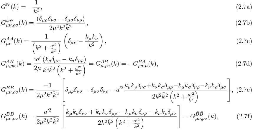
From the action (2.6) with J/J¯and Q/Q¯ set to their physical values given by (2.5) one finds the propagators
G¯cc(k) =− 1
k2, (2.7a)
Gψψµν,ρσ¯ (k) =
(δµρδνσ−δµσδνρ)
2µ2k2˜k2 , (2.7b)
GAAµν (k) = 1
k2+a′2
˜
k2
δµν−
kµkν
k2
, (2.7c)
GABµ,ρσ(k) = ia ′ 2µ
(kρδµσ−kσδµρ)
k2˜k2k2+a′2
˜
k2
=GAµ,ρσB¯ (k) =−GBAρσ,µ¯ (k), (2.7d)
GBBµν,ρσ¯ (k) = −1 2µ2k2k˜2
δµρδνσ−δµσδνρ−a′2
kµkρδνσ+kνkσδµρ−kµkσδνρ−kνkρδµσ
2k2k˜2k2+a′2
˜
k2
, (2.7e)
GBBµν,ρσ(k) = a ′2
2µ2k2k˜2
kµkρδνσ +kνkσδµρ−kµkσδνρ−kνkρδµσ
2k2k˜2k2+a′2
˜
k2
=GBµν,ρσ¯B¯ (k), (2.7f)
where the abbreviation a′ ≡λ/µis used. Notice, that they obey the following symmetries and relations:
GABµ,ρσ(k) =GAµ,ρσB¯ (k) =−GBAρσ,µ(k) =−GBAρσ,µ¯ (k), (2.8a)
Gφµν,ρσ(k) =−Gφνµ,ρσ=−Gφµν,σρ(k) =Gνµ,σρφ (k), for φ∈ {ψψ,¯ BB, BB,¯ B¯B¯}, (2.8b)
2k2k˜2GABρ,µν(k) = ia ′ µ kµG
AA
ρν (k)−kνGAAρµ (k)
, (2.8c)
1
µ2(δµρδνσ−δµσδνρ) = i
a′ µ kµG
BA
ρσ,ν(k)−kνGBAρσ,µ(k)
−2k2k˜2GBµν,ρσB¯ (k), (2.8d)
0 = ia ′ µ kµG
BA
ρσ,ν(k)−kνGBAρσ,µ(k)
−2k2˜k2GBBµν,ρσ(k), (2.8e)
GBµν,ρσB¯ (k) =G
¯
ψψ
2.2.2 Vertices
The action (2.6) leads to 13 tree level vertices whose rather lengthy expressions are listed in AppendixA. One immediately finds the following vertex relation:
e
i.e. all vertices with oneB, one ¯B and an arbitrary number ofAlegs have exactly the same form as the ones with one ψ, one ¯ψ and an arbitrary number ofA legs. This is due to the fact that the ¯ψψnAand ¯BBnA vertices stem from terms in the action which are of the same structure, and are thus equal in their form.
Finally, the vertices obey the following additional relations:
e
Before moving on to explicit one-loop calculations, let us briefly discuss the symmetries of our action equation (2.6). The Slavnov–Taylor identity is given by
B(S) =
Furthermore we have the gauge fixing condition
δS
and the antighost equation
¯ G(S) =
Z
d4xδS δc = 0.
Following the notation of [2] the identity associated to the BRST doublet structure is given by
+Jµνρσ
Note that the first two terms of the second line,
Z
constitute a symmetry by themselves. These terms stem from the insertion of conjugated field partners J and Q for ¯J and ¯Q, respectively, which are not necessarily required as discussed above in Section 2.1.
Furthermore, we have the linearly broken symmetriesU(0) and ˜U(0):
Uαβµν(0) (S) =−Θ(0)αβµν =−U˜αβµν(0) (S),
The above relations would, if applicable, form the starting point for the algebraic renormalization procedure. In order to assure the completeness of the set of symmetries it has to be assured that the algebra generated by them closes. From the Slavnov–Taylor identity (2.9) one derives the linearized Slavnov operator
BS =
Furthermore, the U(0) and ˜U(0) symmetries are combined to define the operator Q as
Q ≡δαµδβν Uαβµν(0) + ˜Uαβµν(0)
.
Having defined the operators BS, ¯G, Q and U(1) we may derive the following set of graded
commutators:
¯
G,G¯ = 0, {BS,BS}= 0, {G¯,BS}= 0,
¯
G,Q= 0, [Q,Q] = 0, G¯,Uµναβ(1) = 0,
BS,Uµναβ(1) = 0,
Uµναβ(1) ,Uµ(1)′ν′α′β′ = 0,
Uµναβ(1) ,Q= 0,
[BS,Q] = 0,
which shows that the algebra of symmetries closes.
Having derived the symmetry content of the model, we would now be ready to apply the method of Algebraic Renormalization (AR). The latter requires locality which, however, is not given in the present case and generally for all commutative QFTs, due to the inherent non-locality of the star product. Hence, before the application of AR it would be required to establish the foundations of this method also for non-commutative theories. For a detailed discussion we would like to refer to our recent article [22].
3
One-loop calculations
In this section we shall present the calculations relevant for the one-loop correction to the gauge boson propagator. Due to the existence of the mixed propagatorsGAB,GA ¯B, and their mirrored
counterparts, the two point function hAµAνi receives contributions not only from graphs with
external gauge boson legs, but also from those featuring externalB and/or ¯B fields.
In the following (i.e. in Sections3.1–3.4), we will present a detailed analysis of all truncated two-point functions relevant for the calculation of the full one-loopAA-propagator. Every type of correction, being characterized by its amputated external legs (i.e. A, B or ¯B), is discussed in a separate subsection. Finally, in Section3.5the dressedAA-propagator and the attempt for its one-loop renormalization will be given explicitly.
3.1 Vacuum polarization
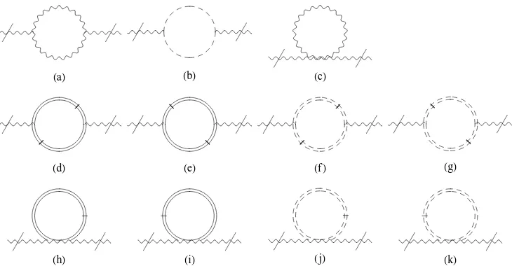
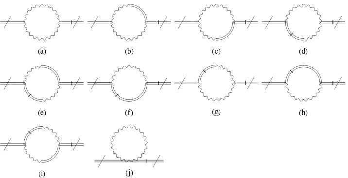
The model (2.6) gives rise to 23 graphs contributing to the two-point functionGAAµν (p). Omitting
convergent expressions, there are 11 graphs left depicted in Fig. 1. Being interested in the divergent contributions one can apply the expansion [3]
Πµν =
Z
d4kIµν(p, k) sin2
kp˜ 2
≈
Z
d4k sin2k2p˜ Iµν(0, k) +pρ
∂pρIµν(p, k)
p=0
+pρpσ 2
∂pρ∂pσIµν(p, k)
p=0+O p 3
, (3.1)
where the integrand Iµν(p, k) has been separated from the phase factor in order to keep the
regularizing effects in the non-planar parts due to rapid oscillations for large k. Summing up the contributions of the graphs in Fig. 1 and denoting the result at order i for the planar (p) part by Π(µνi),p, one is left with
Π(0)µν,p(p) = g
2
16π2Λ 2δ
µν(−10sc−96sh−96sj+ 12sa+sb+ 96sd+ 96sf) = 0,
Π(2)µν,p(p) =−1 3
g2 16π2
h
δµνp2(22sa+sb+ 48(sd+sf))
+ 2pµpν(72(sh+sj)−8sa+sb−96(sd+sf)) i
K0 2 r
M2
HaL HbL HcL
HdL HeL HfL HgL
HhL HiL HjL HkL
Figure 1. One loop corrections for the gauge boson propagator.
Table 2. Symmetry factors for the one loop vacuum polarization (where the factor (−1) for fermionic loops has been included).
sa 12 se 1 si 1
sb −1 sf −1 sj −1
sc 12 sg −1 sk −1
sd 1 sh 1
=− 5g
2
12π2 p 2δ
µν−pµpν
K0 2 r
M2
Λ2 !
≈ − 5g
2
24π2 p 2δ
µν−pµpν
ln
Λ2
M2
+ finite,
where the symmetry factors in Table 2have been inserted and the approximation
K0(x) ≈
x≪1ln 2
x−γE+O x
2,
for the modified Bessel function K0 can be utilized for small arguments, i.e. vanishing regulator
cutoffs2 Λ → ∞ and M → 0. Finally, γE denotes the Euler–Mascheroni constant. Note that
the first order vanishes identically due to an odd power of k in the integrand which leads to a cancellation under the symmetric integration over the momenta.
Of particular interest is the non-planar part (np) which for smallp results to:
Π(0)µν,np(p) = g
2
4π2p˜2 h
δµν(96(sh+sj−sd−sf)−12sa−sb+ 10sc)
−2p˜µp˜ν ˜
p2 (48(sh+sj)−96(sd+sf)−12sa−sb+ 2sc) i
= 2g
2
π2
˜ pµp˜ν
(˜p2)2, (3.2a)
Π(2)µν,np(p) = g
2
48π2p˜2
2θ2pµpνp2(72(sh+sj)−8sa+sb−96(sd+sf)) K0 p
M2p˜2
+
r
˜ p2
M2p 2
r
˜ p2
M2(22sa+sb+ 48(sd+sf))M 2δ
µνK0 p
M2p˜2
2
The cutoffs are introduced via a factor exp
−M 2
α− 1 Λ2α
to regularize parameter integralsR∞
HaL HbL HcL HdL
HeL HfL HgL HhL
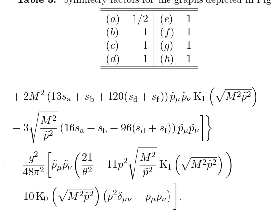
Figure 2. One loop corrections forhAµBν1ν2i(with amputated external legs).
Table 3. Symmetry factors for the graphs depicted in Fig.2. (a) 1/2 (e) 1
(b) 1 (f) 1
(c) 1 (g) 1
(d) 1 (h) 1
+ 2M2(13sa+sb+ 120(sd+sf)) ˜pµp˜νK1 p
M2p˜2
−3
s
M2
˜
p2 (16sa+sb+ 96(sd+sf)) ˜pµp˜ν
=− g
2
48π2
˜ pµp˜ν
21 θ2 −11p
2 s
M2
˜ p2 K1
p
M2p˜2
−10 K0 p
M2p˜2 p2δ
µν−pµpν
. (3.2b)
Considering the limit ˜p2 →0 rectifies application of the approximation
K1(x) ≈
x≪1 1
x + x
2 γE−12 + lnx2
+O x2,
which reveals that the second order is IR finite (which is immediately clear from the fact that the terms of lowest order in pare O p2), apart from a ln(M2)-term which cancels in the sum
of planar and non-planar contributions. Hence, collecting all divergent terms one is left with (in the limit M →0 and Λ→ ∞),
Πµν(p) =
2g2
π2
˜ pµp˜ν
(˜p2)2 −Λlim→∞
5g2
24π2 p 2δ
µν−pµpν
ln Λ2+ finite terms, (3.3)
which is independent of the IR-cutoffM. As expected3, equation (3.3) exhibits a quadratic IR divergence in ˜p2 and a logarithmic divergence in the cutoff Λ. Furthermore, the transversality
conditionpµΠµν(p) = 0 is fulfilled, which serves as a consistency check for the symmetry factors.
3.2 Corrections to the AB propagator
The action (2.6) gives rise to eight divergent graphs with one externalAµ and one Bµν which
are depicted in Fig. 2. Applying an expansion of type (3.1) for small external momenta p and
3
HaL HbL HcL HdL
HeL HfL HgL HhL
HiL
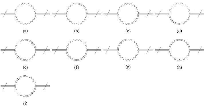
Figure 3. One loop corrections forhBµ1µ2Bν1ν2i(with amputated external legs).
Table 4. Symmetry factors for the graphs depicted in Fig.3. (a) 1/2 (d) 1 (g) 1
(b) 1 (e) 1 (h) 1 (c) 1 (f) 1 (i) 1
summing up the divergent contributions of all graphs (all orders of an expansion similar to equation (3.1)) one ends up with,
Σp,ABµ1,ν1ν2(p) =−3ig
2
32π2λ(pν1δµ1ν2−pν2δµ1ν1) K0 2 r
M2
Λ2 !
+ finite,
Σnp,ABµ1,ν1ν2(p) = 3ig
2
32π2λK0 p
M2p˜2(p
ν1δµ1ν2−pν2δµ1ν1) + finite.
Approximating the Bessel functions as in Section 3.1 and summing up planar and non-planar parts one finds the expression
ΣABµ1,ν1ν2(p) = 3ig
2
32π2λ(pν1δµ1ν2−pν2δµ1ν1) (ln Λ + ln|p˜|) + finite,
where the IR cutoff M has cancelled, and which shows a logarithmic divergence for Λ→ ∞. Due to the symmetry between B and ¯B in the sense that both have identical interactions with the gauge field, it is obvious that ΣABµ1,ν1ν2 ≡ΣA ¯B
µ1,ν1ν2 and as implied by equation (2.8a) it
also holds that ΣBA
µ1µ2,ν1≡ −ΣABν1,µ1µ2.
3.3 Corrections to the BB propagator
The set of divergent graphs contributing to hBµ1µ2Bν1ν2i consists of those depicted in Fig. 3.
Making an expansion of type (3.1) for small external momentap and summing up the contribu-tions of all nine graphs yields
Σp,BBµ1µ2,ν1ν2(p) = g
2λ2
32π2(δµ1ν1δµ2ν2−δµ2ν1δµ1ν2) K0 2 r
M2
Λ2 !
+ finite,
Σnp,BBµ1µ2,ν1ν2(p) = g
2λ2
64π2
δµ1ν2p˜µ2p˜ν1−δµ1ν1p˜µ2p˜ν2−δµ2ν2p˜µ1p˜ν1+δµ2ν1p˜µ1p˜ν2
HaL HbL HcL HdL
HeL HfL HgL HhL
HiL HjL
Figure 4. One loop corrections forhBµ1µ2Bν¯ 1ν2i(with amputated external legs).
Table 5. Symmetry factors for the graphs depicted in Fig.4. (a) 1/2 (e) 1 (i) 1
(b) 1 (f) 1 (j) 1/2
(c) 1 (g) 1
(d) 1 (h) 1
+ 2 K0 p
M2p˜2(δ
µ1ν2δµ2ν1−δµ1ν1δµ2ν2)
+ finite,
for the planar/non-planar part, respectively. Approximating the Bessel functions as in Sec-tion 3.1 reveals cancellations of contributions depending on M in the final sum. Hence, the divergent part boils down to
ΣBBµ1µ2,ν1ν2(p) = g
2λ2
64π2(δµ1ν1δµ2ν2−δµ2ν1δµ1ν2) ln Λ
2+ ln ˜p2+ finite, (3.4)
leaving a logarithmic divergence for both the planar and the non-planar part. Due to symmetry reasons this result is also equal to the according correction to the ¯BB¯ propagator, i.e.
ΣB ¯µ¯1Bµ2,ν1ν2(p) = ΣBBµ1µ2,ν1ν2(p).
3.4 Corrections to the BB¯ propagator
For the correction to hBµ1µ2B¯ν1ν2i one finds the ten divergent graphs depicted in Fig. 4.
Ex-pansion for small external momenta pand summation of the integrated results yields
Σpµ,1B ¯µB2,ν1ν2(p) = g
2
2π2Λ
2µ2p˜2(δ
µ2ν1δµ1ν2−δµ1ν1δµ2ν2)
+ g
2λ2
32π2 (δµ1ν1δµ2ν2−δµ2ν1δµ1ν2) K0 2 r
M2
Λ2 !
+ finite,
Σnpµ1,µB ¯2B,ν1ν2(p) = g
2λ2
64π2
δµ1ν2p˜µ2p˜ν1−δµ1ν1p˜µ2p˜ν2−δµ2ν2p˜µ1p˜ν1+δµ2ν1p˜µ1p˜ν2
˜ p2
+ 2 K0 p
M2p˜2(δ
µ1ν2δµ2ν1−δµ1ν1δµ2ν2)
Hence, the divergent part is given by
ΣB ¯µ1Bµ2,ν1ν2(p) = g
2
2π2Λ
2µ2p˜2(δ
µ2ν1δµ1ν2−δµ1ν1δµ2ν2)
+ g
2λ2
64π2 (δµ1ν1δµ2ν2−δµ2ν1δµ1ν2) ln Λ
2+ ln ˜p2+ finite,
which is logarithmically divergent in ˜p2and quadratically in Λ. Once more,M has dropped out in the sum of planar and non-planar contributions. Furthermore, note that ΣB ¯µ1Bµ2,ν1ν2≡ΣBBν¯1ν2,µ1µ2 as is obvious from the result (3.4).
3.5 Dressed gauge boson propagator and analysis
In the standard renormalization procedure, the dressed propagator at one-loop level is given by
≡∆′(p) = 1 A +
1
AΣ(Λ, p) 1
A, (3.5)
where 1 A ≡G
AA
µν(p), Σ(Λ, p)≡ Πplan
regul.(Λ, p) + Π
n-pl(p).
For A 6= 0, one can apply the formula
1 A+B =
1 A−
1 AB
1 A+B =
1 A −
1 AB
1
A +O(B
2), (3.6)
which allows one to rewrite expression (3.5) to order Σ as
∆′(p) = 1 A −Σ(Λ, p),
and thus (in the case of renormalizability) to absorb any divergences in the appropriate param-eters of the theory present in A(see [14] for an example).
However, in our case (3.6) cannot be applied directly, as the complete one loop correction to the gauge boson propagator is given by the sum of all the results of Sections 3.1–3.4 after multiplication with appropriate, i.e. differentexternal legs:
GAAµν,1l−ren(p) =GAAµν (p) +GAAµρ (p)Πρσ(p)GσνAA(p) +GAAµρ (p)2ΣABρ,σ1σ2(p)GBAσ1σ2,ν(p)
+GAAµρ (p)2ΣA ¯ρ,σB1σ2(p)GBAσ¯1σ2,ν(p) +Gµ,ρAB1ρ2(p)ΣBBρ1ρ2,σ1σ2(p)GBAσ1σ2,ν(p)
+GABµ,ρ1ρ2(p)2ΣB ¯ρ1Bρ2,σ1σ2(p)GBAσ¯1σ2,ν(p) +GA ¯µ,ρB1ρ2(p)ΣB ¯ρ¯1Bρ2,σ1σ2(p)GBAσ¯1σ2,ν(p)
+O g4. (3.7)
Note, that the factors 2 stem from the (not explicitly written) mirrored contributionsAB↔BA, AB¯ ↔BA, and¯ BB¯ ↔BB. Since the factor¯ Amust be the same for all summands we have to use the Ward Identities (2.8a) and (2.8c), i.e.
GABµ,ρσ(k) =GA
¯
B
µ,ρσ(k) =−GBAρσ,µ(k) =−G
¯
BA ρσ,µ(k),
2k2k˜2GABρ,µν(k) = i
a′ µ kµG
AA
ρν (k)−kνGAAρµ (k)
, (3.8)
which allow us to express the (tree level) AB and AB¯ propagators uniquely in terms of AA-propagators. This leads (in analogy to (3.6)) to the following representation for the dressed one-loop gauge boson propagator:
GAAµν,1l−ren(p) = 1 A −
1 A
X
Bi
1
where 1/A once more stands for the tree level gauge boson propagator. The Bi’s are given by
the one-loop corrections (with amputated external legs) of the two-point functions relevant for the dressed gauge boson propagator, multiplied by any prefactors coming from (3.8) and the factor 2 where needed (c.f. (3.7)). Thus, the full propagator is given by
GAAµν,1l−ren(p) =GµνAA(p) +GAAµρ (p)Πρσ(p)GAAσν (p)
+
ia′ µp2p˜2
(
2GAAµρ(p)
ΣABρ,σ1σ2(p) + ΣA ¯ρ,σB1σ2(p)
pσ2GAAνσ1(p)
+µpia2′p˜2
pρ1GAAµρ2(p)
ΣρBB1ρ2,σ1σ2(p) + 2ΣρB ¯1Bρ2,σ1σ2(p) + Σ ¯ B ¯B
ρ1ρ2,σ1σ2(p)
pσ2GAAνσ1(p) )
.
The expression B=P
i
Bi forM →0 is explicitly given by
B= g
2
8π2µ4 (
˜ pµp˜ν
16µ4
(˜p2)2 +
θ4λ4
2(˜p2)4
−7λ2µ2 θ
4
(˜p2)4 p 2δ
µν−pµpν 4−p˜2Λ2
+ p2δµν−pµpν
[ln 2−ln|p˜| −ln Λ]
5 3µ
4+3λ2µ2θ2
(˜p2)2 +
λ4θ4
(˜p2)4 )
+ finite,
and shows us two things: In contrast to commutative gauge models and even though the vacuum polarization tensor Πµνonly had a logarithmic UV divergence, the fullBdiverges quadratically in
the UV cutoff Λ. Secondly, despite the fact that Πµν exhibited the usual quadratic IR divergence,
Bbehaves like (˜p12)3 in the IR limit. Both properties arise due to the existence (and the form) of
the mixed AB and AB¯ propagators, and seem problematic concerning renormalization for two reasons: On the one hand, the form of the propagator is modified implying new counter terms in the effective action. On the other hand, higher loop insertions of this expression can lead to IR divergent integrals, as will be discussed in the next section.
4
Higher loop calculations
In the light of higher loop calculations it is important to investigate the IR behaviour of expected integrands with insertions of the one-loop corrections being discussed in Section3. The aim is to identify possible poles at ˜p2= 0. Hence, we consider a chain ofnnon-planar insertions denoted by Ξφ1φ2(p, n), which may be part of a higher loop graph. Every insertion Ξ represents the sum
of all divergent one-loop contributions with external fieldsφ1 andφ2 (cf. Sections3.1–3.4). Due
to the numerous possibilities of constructing such graphs, we will examine only a few exemplary configurations in this section – especially those for which one expects the worst IR behaviour.
To start with, let us state that amongst all types of two point functions, the vacuum polariza-tion shows the highest, namely a quadratic divergence. Amongst the propagators those with two external double-indexed legs, e.g. B or ¯B feature the highest (quartic) divergence in the limit of vanishing external momenta. A chain ofnvacuum polarizations Πnpµν(p) (see equations (3.2a)
and (3.2b)) with (n+ 1) AA-propagators ((n−1) between the individual vacuum polarization graphs, and one at each end) leads to the following expression (for a graphical representation, see Fig. 5):
ΞAAµν (p, n) = GAA(p)Πnp(p)nµρGAAρν (p) =
2g2
π2
n
1
p2+a′2
˜
p2
n+1
˜ pµp˜ν
pµ
· · ·
1 2 n
pν
Figure 5. A chain ofnnon-planar insertions, concatenated by gauge field propagators.
Note that due to transversality, from the propagator (2.7c) only the term with the Kronecker delta enters the calculation. For vanishing momenta, i.e. in the limit ˜p2 → 0 the expression
reduces to
lim
˜
p2→0Ξ AA
µν (p, n) =
2g2 π2
n
˜ pµp˜ν
a′2(n+1),
exhibiting IR finiteness which is independent from the number of inserted loops. Another representative is the chain
ΞAφ(p, n)≡GAφ(p)Σnp,φA(p)GAφ(p)n, where φ∈ {B,B¯},
which could replace any single GAB (or GAB¯) line. Obviously, one has
ΞAφµ,ν1ν2(p, n) = ia ′ 2µ
− 3g
2
32π2a
′2
n
(pν1δµ ν2−pν2δµ ν1)
p2hp˜2p2+a′2
˜
p2
in+1nln ˜p2,
which for ˜p2 ≪1 (and neglecting dimensionless prefactors) behaves like
ΞAφµ,ν1ν2(p, n)≈n(pν1δµ ν2−pν2δµ ν1) µp2 ln ˜p
2.
The latter insertion can be regularized since the pole at p= 0 is independent ofn. In contrast, higher divergences are expected for chain graphs being concatenated by propagators with four indices, i.e.GBB¯
µν,ρσ,GBBµν,ρσ,G
¯
ψψ
µν,ρσ, due to the inherent quartic IR singularities. Let us start with
the combination ΞBB¯ (p, n) ≡ GBB¯ (p)Σp,B ¯B(p)n
GBB¯ (p). As before, we can approximate for
˜
p2 ≪1 and, omitting dimensionless prefactors and indices, find
ΞAφ(p, n) ∝
˜
p2≪1
n µ2
ln ˜p2 (p2p˜2)n,
which represents a singularity∀n >1 (since in any graph, atn= 0, the divergence is regularized by the phase factor being a sine function which behaves like p for small momenta). Regarding the index structures, no cancellations can be expected since the product of an arbitrary num-ber of contracted, completely antisymmetric tensors is again an antisymmetric tensor with the outermost indices of the chain being free.
Exactly the same result is obtained for ΞBB(p)≡ GBB(p)Σp,BB(p)nGBB(p). From this it is clear that the damping mechanism seen in ΞAA(p, n) fails for higher insertions of B/B¯ (and
also ψ/ψ) fields).¯
5
Discussion
of the theory which is the basis for the generation of constraints to potential counter terms. Therefore, after recapitulating general properties of our model, we studied the resulting algebra of symmetries. However, as we exposed recently [22], the foundations of AR are only proved to be valid inlocalQFTs so far, and hence may not be applicable in non-commutative field theories, as the deformation inherently implies non-locality. In order to find a way out of this dilemma, explicit loop-calculations were presented, and our hope was to show renormalizability – at least at the one-loop level. In this respect, unexpected difficulties appeared. The soft breaking term, being required to implement the IR damping behaviour of the 1/p2 model in a way being
compatible with the Quantum Action Principle of AR, gives rise to mixed propagators GAB and GAB¯. These, in turn, allow the insertion of one-loop corrections with externalB-fields into
the dressedAApropagator (see Section4) and, therefore, enter the renormalization. Despite all corrections featuring the expected p˜12 IR behaviour, the dressed propagators with external AB
or AB¯ legs multiplicatively receive higher poles due to the inherent quadratic divergences in GAB(p) (andGAB¯(p)) forp→0. As a consequence, the resulting corrections cannot be absorbed
in a straightforward manner.
However, renormalizability of the non-local model (1.1) cannot depend on how it is localized due to equivalence of the respective path integrals (see [17]). Therefore, we expect the same problems to appear inall localized versions of (1.1), including the one of Vilar et al. [2]. In fact, from the discussion in Appendix B, one notices that the propagators (B.2f)–(B.2h) and (B.2s) of their action all exhibit the same quartic IR divergences as those of our present model (2.6), even though the operatorDµ appears at most quadratically asD2 in the according action (B.1).
Nonetheless, the authors claim to have shown renormalizability using Algebraic Renormalization, which as we have discussed in [22] may not be applicable in non-commutative theories.
In this respect it has to be noted that in commutative space the model of Vilar et al. [2] should indeed be renormalizable, since the action, apart from the star product, is completely local and provides the necessary symmetries for the Quantum Action Principle. Since the propagators are the same in both spaces, and hence show the same quartic IR divergences, one may expect related IR problems to cancel when considering the sum of bosonic and fermionic sectors (i.e.B/χandψ/ξ). These cancellations should also take place in non-commutative space (in both models), but the problem of proving renormalization remains (cf. Section3.5).
Coming back to the problem of IR divergent propagators we have also investigated the struc-ture of singularities in higher-loop integrands by studying chain graphs consisting of interleav-ing tree-level propagators, and one-loop corrections of various types. It turned out that chains containing gauge fields benefit from the damping of the propagator (2.7c) while those con-sisting (solely) of concatenated B and ¯B fields and insertions do (expectedly) not. Hence, at first sight, there exist divergences which increase order by order, which would indicate non-renormalizability. However, we may point out that, due to the symmetry between the B/B¯ and ψ/ψ¯sectors, cancellations can be expected. These already appear in our one-loop calculations, and there is strong evidence that they appear to all orders. An intuitive argument can be given when considering the action (2.2) for λ → 0, i.e. vanishing damping. In this case, the B/B¯ and ψ/ψ¯ fields may simply be integrated out in the path integral formalism (see [17]), and the contributions cancel exactly. An alternative approach which avoids these uncertainties is in preparation.
A
Vertices
k2,σ
k1,ρ
k3,τ
=Veρστ3A(k1, k2, k3) = 2ig(2π)4δ4(k1+k2+k3) sin
k1˜k2
2
×
B
Propagators of the model by Vilar et al.
The tree level action of [2] is given by:
of this action one derives the following 19 propagators:
GχBρσ,τ ǫ(k) = γ
4
k2
(kρkτδσǫ+kσkǫδρτ −kρkǫδστ −kσkτδρǫ)
4(k2)2k2+γ4 k2
, (B.2l)
Gχρσ,τ ǫ¯B¯ (k) =GχBρσ,τ ǫ(k), (B.2m)
Gχρσ,τ ǫB¯ (k) = (δρτδσǫ−δρǫδστ)
2k2 −G
χB
ρσ,τ ǫ(k), (B.2n)
GχBρσ,τ ǫ¯ (k) =Gχρσ,τ ǫB¯ (k), (B.2o)
G¯cc(k) =− 1
k2, (B.2p)
Gξ,µν,ρσψ¯ (k) =
(δµρδνσ−δµσδνρ)
2k2 , (B.2q)
Gξ,ψµν,ρσ¯ (k) =−Gξ,
¯
ψ
µν,ρσ, (B.2r)
Gξξµν,ρσ¯ (k) =−γ2(δµρδνσ−δµσδνρ)
2(k2)2 . (B.2s)
Acknowledgements
The authors are indebted to M. Schweda and M. Wohlgenannt for valuable discussions. The work of D.N. Blaschke, A. Rofner and R.I.P. Sedmik was supported by the “Fonds zur F¨orderung der Wissenschaftlichen Forschung” (FWF) under contract P20507-N16.
References
[1] Gurau R., Magnen J., Rivasseau V., Tanasa A., A translation-invariant renormalizable non-commutative scalar model,Comm. Math. Phys.287(2009), 275–290,arXiv:0802.0791.
[2] Vilar L.C.Q., Ventura O.S., Tedesco D.G., Lemes V.E.R., On the renormalizability of noncommutative
U(1) gauge theory – an algebraic approach, J. Phys. A: Math. Theor. 43 (2010), 135401, 13 pages, arXiv:0902.2956.
[3] Blaschke D.N., Rofner A., Schweda M., Sedmik R.I.P., One-loop calculations for a translation invariant non-commutative gauge model,Eur. Phys. J. C: Part. Fields62(2009), 433–443,arXiv:0901.1681. [4] Minwalla S., Van Raamsdonk M., Seiberg N., Noncommutative perturbative dynamics,J. High Energy Phys.
2000(2000), no. 2, 020, 30 pages,arXiv:hep-th/9912072.
[5] Matusis A., Susskind L., Toumbas N., The IR/UV connection in the non-commutative gauge theories,
J. High Energy Phys.2000(2000), no. 12, 002, 18 pages,hep-th/0002075.
[6] Tanasa A., Scalar and gauge translation-invariant noncommutative models,Romanian J. Phys.53(2008) 1207–1212,arXiv:0808.3703.
[7] Rivasseau V., Non-commutative renormalization, in Quantum Spaces – Poincar´e Seminar 2007, Edi-tors B. Duplantier and V. Rivasseau, Prog. Math. Phys., Vol. 53, Birkh¨auser, Basel, 2007, 19–107, arXiv:0705.0705.
[8] Douglas M.R., Nekrasov N.A., Noncommutative field theory, Rev. Modern Phys. 73 (2001), 977–1029, hep-th/0106048.
[9] Grosse H., Wulkenhaar R., Renormalisation ofφ4
theory on noncommutativeR2
in the matrix base,J. High Energy Phys.2003(2003), no. 12, 019, 26 pages,hep-th/0307017.
[10] Grosse H., Vignes-Tourneret F., Quantum field theory on the degenerate Moyal space,arXiv:0803.1035.
[11] Rivasseau V., Vignes-Tourneret F., Wulkenhaar R., Renormalization of noncommutativeφ4-theory by multi-scale analysis,Comm. Math. Phys.262(2006), 565–594,hep-th/0501036.
[12] Gurau R., Magnen J., Rivasseau V., Vignes-Tourneret F., Renormalization of non-commutative Φ4 4 field theory inxspace,Comm. Math. Phys.267(2006), 515–542,hep-th/0512271.
[13] Grosse H., Wulkenhaar R., Renormalisation ofφ4
[14] Blaschke D.N., Gieres F., Kronberger E., Reis T., Schweda M., Sedmik R.I.P., Quantum corrections for translation-invariant renormalizable non-commutativeφ4
theory,J. High Energy Phys.2008(2008), no. 11, 074, 16 pages,arXiv:0807.3270.
[15] Ben Geloun J., Tanasa A., One-loopβfunctions of a translation-invariant renormalizable noncommutative scalar model,Lett. Math. Phys.86(2008), 19–32,arXiv:0806.3886.
[16] Blaschke D.N., Gieres F., Kronberger E., Schweda M., Wohlgenannt M., Translation-invariant models for non-commutative gauge fields,J. Phys. A: Math. Theor.41(2008), 252002, 7 pages,arXiv:0804.1914. [17] Blaschke D.N., Rofner A., Schweda M., Sedmik R.I.P., Improved localization of a renormalizable
non-commutative translation invariant U(1) gauge model, Europhys. Lett. 86 (2009), 51002, 6 pages, arXiv:0903.4811.
[18] Zwanziger D., Local and renormalizable action from the Gribov horizon, Nuclear Phys. B 323 (1989), 513–544.
[19] Zwanziger D., Renormalizability of the critical limit of lattice gauge theory by BRS invariance, Nuclear Phys. B399(1993), 477–513.
[20] Dudal D., Gracey J., Sorella S.P., Vandersickel N., Verschelde H., A refinement of the Gribov–Zwanziger approach in the Landau gauge: infrared propagators in harmony with the lattice results,Phys. Rev. D78 (2008), 065047, 30 pages,arXiv:0806.4348.
[21] Baulieu L., Sorella S.P., Soft breaking of BRST invariance for introducing non-perturbative infrared effects in a local and renormalizable way,Phys. Lett. B671(2009), 481–485,arXiv:0808.1356.
[22] Blaschke D.N., Kronberger E., Rofner A., Schweda M., Sedmik R.I.P., Wohlgenannt M., On the problem of renormalizability in non-commutative gauge field models – a critical review,Fortschr. Phys.58(2010), 364–372,arXiv:0908.0467.
[23] Hayakawa M., Perturbative analysis on infrared aspects of noncommutative QED onR4,Phys. Lett. B478 (2000), 394–400,hep-th/9912094.
[24] Armoni A., Comments on perturbative dynamics of non-commutative Yang–Mills theory,Nuclear Phys. B
593(2001), 229–242,hep-th/0005208.
[25] Ruiz Ruiz F., Gauge-fixing independence of IR divergences in non-commutativeU(1), perturbative tachyonic instabilities and supersymmetry,Phys. Lett. B502(2001), 274–278,hep-th/0012171.