The Symmetrical
H
q-Semiclassical
Orthogonal Polynomials of Class One
Abdallah GHRESSI † and Lotf i KH ´ERIJI ‡
† Facult´e des Sciences de Gab`es, Route de Mednine 6029 Gab`es, Tunisia
E-mail: [email protected]
‡ Institut Sup´erieur des Sciences Appliqu´ees et de Technologies de Gab`es,
Rue Omar Ibn El-Khattab 6072 Gab`es, Tunisia E-mail: [email protected]
Received December 12, 2008, in final form July 07, 2009; Published online July 22, 2009 doi:10.3842/SIGMA.2009.076
Abstract. We investigate the quadratic decomposition and duality to classify symmetrical
Hq-semiclassical orthogonal q-polynomials of class one where Hq is the Hahn’s operator. For any canonical situation, the recurrence coefficients, the q-analog of the distributional equation of Pearson type, the moments and integral or discrete representations are given.
Key words: quadratic decomposition of symmetrical orthogonal polynomials; semiclassical form; integral representations; q-difference operator; q-series representations; theq-analog of the distributional equation of Pearson type
2000 Mathematics Subject Classification: 33C45; 42C05
1
Introduction
Orthogonal polynomials (OP) have been a subject of research in the last hundred and fifty years. The orthogonality considered in our contribution is related to a form (regular linear functional) [8, 24] and not only to a positive measure. By classical orthogonal polynomials sequences (OPS), we refer to Hermite, Laguerre, Bessel and Jacobi polynomials. In the liter-ature, the extension of classical (OPS) can be done from different approaches such that the hypergeometric character [7, 8, 11, 18, 22] and the distributional equation of Pearson type [6, 8, 20, 29, 32]. A natural generalization of the classical character is the semiclassical one introduced by J.A. Shohat in [35]. This theory was developed by P. Maroni and extensively studied by P. Maroni and coworkers in the last decade [1,24,26,28,32]. Let Φ monic and Ψ be two polynomials, deg Φ =t≥0, deg Ψ =p≥1. We suppose that the pair (Φ,Ψ) is admissible, i.e., when p = t−1, writing Ψ(x) = apxp+· · ·, then ap 6=n+ 1, n ∈ N. A form u is called semiclassical when it is regular and satisfies the distributional equation of Pearson type
D(Φu) + Ψu= 0, (1.1)
where the pair(Φ,Ψ) is admissible and D is the derivative operator. The corresponding monic orthogonal polynomials sequence (MOPS) {Bn}n≥0 is called semiclassical. Moreover, if u is semiclassical satisfying (1.1), the class of u, denoted sis defined by
s:= min max(deg Φ−2,deg Ψ−1)≥0,
where the minimum is taken over all pairs (Φ,Ψ) satisfying (1.1). In particular, whens= 0 the classical case is recovered.
1) The generalized Hermite formH(µ) (µ6= 0,µ=6 −n−12,n≥0) satisfying the distributional equation of Pearson type
D(xH(µ)) + 2x2−(2µ+ 1)H(µ) = 0. (1.2)
2) The generalized Gegenbauer G(α, β) (α6=−n−1,β 6=−n−1,β 6=−12,α+β 6=−n−1,
n≥0) satisfying the distributional equation of Pearson type
D x x2−1G(α, β)+ −2(α+β+ 2)x2+ 2(β+ 1)G(α, β) = 0. (1.3)
For further properties of the generalized Hermite and the generalized Gegenbauer polyno-mials see [8,15,26].
3) The form B[ν] of Bessel kind (ν 6= −n−1, n ≥ 0) [1, 31] satisfying the distributional equation of Pearson type
D x3B[ν]− 2(ν+ 1)x2+12B[ν] = 0. (1.4)
For an integral representation of B[ν] and some additional features of the associated (MOPS) see [14].
Other families of semiclassical orthogonal polynomials of class greater than one were discov-ered by solving functional equations of the typeP(x)u=Q(x)v, whereP,Qare two polynomials cunningly chosen andu,v two linear forms [19,26,27,34]. For other relevant works in the semi-classical case see [5,23].
In [21], instead of the derivative operator, the q-difference one is used to establish the theo-ry and characterizations of Hq-semiclassical orthogonal q-polynomials. Some examples of H q-semiclassical orthogonalq-polynomials are given in [2,13]. TheHq-classical case is exhaustively described in [20,32]. Moreover, in [30] the symmetricalDω-semiclassical orthogonal polynomials of class one are completely described by solving the system of their Laguerre–Freud equations where Dw is the Hahn’s operator.
So, the aim of this paper is to present the classification of the symmetricalHq-semiclassical orthogonal q-polynomials of class one by investigating the quadratic operatorσ, the q-analog of the distributional equation of Pearson type satisfied by the corresponding form and some H q-classical situations (see Tables 1 and 2) in connection with our problem. Among the obtained canonical cases, three are well known: two symmetrical Brenke type (MOPS) [8, 9, 10] and a symmetrical case of the Al-Salam and Verma (MOPS) [2]. Also, q-analogues ofH(µ),G(α, β) and B[ν] appear. In [3,33], the authors have established, up a dilation, a q-analogues ofH(µ) and B[ν] using other methods. For any canonical case, we determine the recurrence coefficient, theq-analog of the distributional equation of Pearson type, the moments and a discrete measure or an integral representation.
2
Preliminary and f irst results
2.1 Preliminary and notations
Let P be the vector space of polynomials with coefficients in C and let P′ be its topological
dual. We denote by hu, fi the effect of u ∈ P′ on f ∈ P. In particular, we denote by (u)n := hu, xni, n≥0 the moments of u. Moreover, a form (linear functional) u is called symmetric if (u)2n+1 = 0,n≥0.
Let us introduce some useful operations in P′. For any form u, any polynomial g and any
Continuation of Table1. Consequently, we define σu by duality [8,25]
hσu, fi:=hu, σfi, f ∈ P, u∈ P′.
We have the well known formula [25]
Continuation of Table1.
Lastly, let us recall the following standard expressions [8,11,20]
Continuation of Table1.
2.2 Some results about the Hq-semiclassical character
A formuis calledHq-semiclassical when it is regular and there exist two polynomials Φ and Ψ, Φ monic, deg Φ =t≥0, deg Ψ =p≥1 such that
Hq(Φu) + Ψu= 0, (2.5)
TheHq-semiclassical character is kept by a dilation [21]. In fact, let{a−n(haBn)}n≥0,a6= 0; when u satisfies (2.5), thenha−1u fulfills theq-analog of the distributional equation of Pearson type
Hq a−tΦ(ax)ha−1u
+a1−tΨ(ax)ha−1u= 0,
and the recurrence coefficients of (2.3) are
βn
a ,
γn+1
a2 , n≥0.
Also, the Hq-semiclassical form u is said to be of class s = max(p−1, t−2) ≥ 0 if and only if [21]
Y
c∈ZΦ
q(hqΨ)(c) + (HqΦ)(c)+hu, q(θcqΨ) + (θcq◦θcΦ)i
>0, (2.6)
where ZΦ is the set of zeros of Φ. In particular, when s = 0 the form u is usually called
Hq-classical (Al-Salam–Carlitz, big q-Laguerre, q-Meixner, Wall, . . . ) [20].
Lemma 1 ([21]). Let ube a symmetrical Hq-semiclassical form of class ssatisfying (2.5). The following statements holds
i) If s is odd then the polynomialΦ is odd and Ψis even.
ii) If s is even then the polynomial Φ is even and Ψis odd.
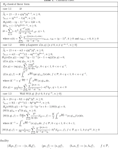
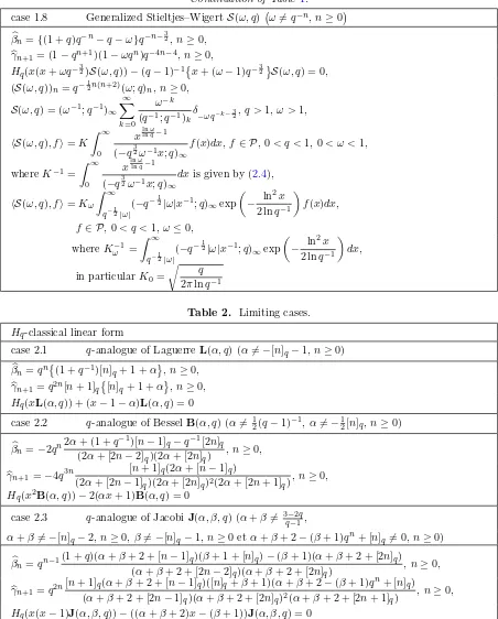
In the sequel we are going to use someHq-classical forms [20], resumed in Table1(canonical cases: 1.1–1.8) and Table 2 (limiting cases: 2.1–2.3). In fact, whenq →1 in results of Table2, we recover the classical Laguerre L(α), Bessel B(α) and h−1
2 ◦τ−1J(α, β) respectively where
J(α, β) is the Jacobi classical form [24].
Moreover in what follows we are going to use the logarithmic function denoted by Log :
C\ {0} −→Cdefined by
Logz= ln|z|+iArgz, z∈C\ {0}, −π <Argz≤π,
Log is the principal branch of log and includes ln :R+\{0} −→Ras a special case. Consequently,
the principal branch of the square root is
√
z=p|z|eiArg z2 , z∈C\ {0}, −π <Argz≤π.
2.3 On quadratic decomposition of a symmetrical regular form
Let u be a symmetrical regular form and {Bn}n≥0 be its MOPS satisfying (2.3) with βn = 0,
n≥0.It is very well known (see [8,25]) that
B2n(x) =Pn x2
, B2n+1(x) =xRn x2
, n≥0,
where{Pn}n≥0 and{Rn}n≥0 are the two MOPS related to the regular formσuandxσu respec-tively. In fact, [8,25]
u is regular⇔ σu andxσuare regular,
Furthermore, taking
Proposition 1. Let u be a symmetrical regular form. (i) The moments of u are
(u)2n= (σu)n, (u)2n+1 = 0, n≥0. (2.10)
(ii) If σu has the discrete representation
σu=
then a possible discrete measure of u is
u=
(iii) If u is positive definite andσu has the integral representation
hσu, fi=
then, a possible integral representation of u is
hu, fi=
Z ∞
−∞|
Proof . (i) is a consequence from the definition of the quadratic operator σ. For (ii) taking into account (2.10), (2.11) we get
(u)2n= (σu)n=
∞ X
k=0
ρk(√τk)2n=
∞ X
k=0
ρk
(√τk)2n+ (
−√τk)2n
2 .
But
(u)2n+1 = 0 =
∞ X
k=0
ρk
(√τk)2n+1+ (−√τk)2n+1
2 .
Hence the desired result (2.12) holds.
For (iii) considerf ∈ P and let us split up the polynomialf accordingly to its even and odd parts
f(x) =fe x2+xfo x2. (2.15)
Therefore since uis a symmetrical form
hu, f(x)i=hu, fe x2i=hσu, fe(x)i. (2.16)
From (2.15) we get
fe(x) = f( √
x) +f(−√x)
2 , x∈R+. (2.17)
By (2.13) and according to (2.16), (2.17) we recover the representation in (2.14).
3
Symmetrical
H
√q-semiclassical orthogonal polynomials
of class one
Lemma 2. We have
σ(Hqu) = (q+ 1)Hq2(σ(xu)), u∈ P′. (3.1)
Proof . From the definition ofHq we get
(Hq(σf))(x) = (q+ 1)x(σ(Hq2f))(x), f ∈ P.
Therefore, ∀f ∈ P,
hσ(Hqu), fi=hHqu, σfi=−hu,(q+ 1)xσ(Hq2f)i
=−h(q+ 1)σ(xu), Hq2fi=h(q+ 1)Hq2(σ(xu)), fi.
Thus the desired result.
Lemma 3. Let u be a symmetrical H√q-semiclassical form of class one. There exist two
poly-nomials ϕ and ψ, ϕmonic, with degϕ≤1 and degψ= 1, such that
H√q xϕ x2u+ψ x2u= 0. (3.2)
Corollary 1. Let u be a symmetricalH√q-semiclassical form of class one satisfying (3.2); then σu et xσu are Hq-classical satisfying respectively the following q-analog of the distributional equation of Pearson type
Hq(xϕ(x)σu) + √ 1
q+ 1ψ(x)σu= 0, (3.3)
Hq(xϕ(x)(xσu)) +q−1
1
√q+ 1ψ(x)−ϕ(x)
(xσu) = 0. (3.4)
Proof . First, σu and xσu are regular because u is symmetrical and regular. Applying the quadratic operatorσ to (3.2) and taking into account (3.1) we get
(√q+ 1)Hq σ x2ϕ x2
u+σ ψ x2u= 0.
By (2.2) we get (3.3). Now, multiplying both sides of (3.3) by q−1x, using the identity in (2.1),
this yields to (3.4).
Regarding Table1 (cases 1.1–1.8), Table 2 (cases 2.1–2.3) and the q-analog of the distribu-tional equation of Pearson type (3.3), (3.4), we consider the following situations for the polyno-mial ϕin order to get a H√q-semiclassical form from aHq-classical
A. ϕ(x) = 1 (cases 1.1,1.2,1.3,1.4,2.1); B. ϕ(x) =x (cases 1.5,2.2); C. ϕ(x) =x−1 (case 2.3); D. ϕ(x) =x−b−1q−1 (case 1.6); E. ϕ(x) =x−µ−1q−1 (case 1.7); F. ϕ(x) =x+ωq−32 (case 1.8).
A. In the case ϕ(x) = 1 the q-analog of the distributional equation of Pearson type (3.3), (3.4) are
Hq(xσu) +√ 1
q+ 1ψ(x)σu= 0, (3.5)
Hq(x(xσu)) +q−1
1
√q+ 1ψ(x)−1
(xσu) = 0. (3.6)
A1. Ifψ(x) = (√q+ 1)(x−1−α) theq-analogue of the Laguerre formL(α, q),α6=−[n]q−1,
n≥0 (case 2.1 in Table2) satisfying
Hq(xL(α, q)) + (x−1−α)L(α, q) = 0.
Comparing with (3.5), (3.6) we get
σu=L(α, q), α6=−[n]q−1, n≥0, (3.7)
and
xσu= (1 +α)L q−1(α+ 2)−1, q, α6=−[n]q−1, n≥0. (3.8)
Taking into account the recurrence coefficients (see case 2.1 in Table2), by virtue of (3.7), (3.8) and (2.7), (2.8) we get forn≥0
βnP =qn 1 +q−1[n]q+ 1 +α , γnP+1 =q2n[n+ 1]q{[n]q+ 1 +α},
With the relation [k−1]q=q−1[k]q−q−1,k≥1 the system (2.9) becomes for n≥0
γ2n+1=qn([n]q+ 1 +α), γ2n+2=qn[n+ 1]q. (3.9)
Writing α =µ− 12,µ 6=−[n]q−12,n≥0 and denoting the symmetrical form u by H(µ, q) we get the following result:
Proposition 2. The symmetrical formH(µ, q) satisfies the following properties: 1) The recurrence coefficient γn+1 satisfies (3.9).
2) H(µ, q) is regular if and only if µ6=−[n]q−12, n≥0. 3) H(µ, q) is positive definite if and only if q >0, µ >−12.
4) H(µ, q) is a H√q-semiclassical form of class one for µ 6= √ 1
q(√q+1) − 12, µ 6= −[n]q −12,
n≥0 satisfying the q-analog of the distributional equation of Pearson type
H√q(xH(µ, q)) + (√q+ 1)
x2−µ−1
2
H(µ, q) = 0. (3.10)
Proof . The results in 1), 2) and 3) are straightforward from (3.9). For 4), it is clear that H(µ, q) satisfies (3.10); in this case and by virtue of (2.6), we are going to prove that the class of H(µ, q) is exactly one for µ 6= √q(√1q+1) − 12, µ 6= −[n]q − 21, n ≥ 0. Denoting Φ(x) = x, Ψ(x) = (√q+ 1) x2−µ−12, we have accordingly to (2.6), on one hand
√q h√ qΨ
(0) + H√qΦ(0) = 1−√q(√q+ 1)
µ+1 2
6
= 0,
and on the other hand by (θ0Ψ)(x) = (√q+ 1)x and (θ20Φ)(x) = 0,
hH(µ, q),√qθ0Ψ +θ02Φi= 0,
taking into account that u is a symmetrical form.
Remark 1. The symmetrical form H(µ, q), µ =6 √q(√1q+1) − 12, µ 6= −[n]q− 12, n ≥ 0 is the
q-analogue of the generalized Hermite one [12] (whenq →1 we recover the generalized Hermite formH(µ) (see (1.2)) which is a symmetrical semiclassical form of class one forµ= 0,6 µ6=−n−12,
n≥0 [1,8,15,26]).
A2. Ifψ(x) =−(√q−1)−1(x+ 1) the formU that satisfies theq-analog of the distributional equation of Pearson type (see case 1.1 in Table 1)
Hq(xU)−(q−1)−1(x+ 1)U = 0.
Comparing with (3.5), (3.6) we get
σu=U, (3.11)
and
xσu=−hqU. (3.12)
Taking into account (3.11), (3.12), (2.7), (2.8) and the case 1.1 in Table 1 we obtain forn≥0
βnP =1−(1 +q)qn qn−1, γnP+1= qn+1−1q3n, βnR=1−(1 +q)qn qn, γnR+1 = qn+1−1q3n+2.
Consequently, the system (2.9) becomes for n≥0
γ2n+1=−q2n, γ2n+2 = 1−qn+1
Proposition 3. The symmetrical formu satisfies the following properties: 1) The recurrence coefficient γn+1 satisfies (3.13).
2) u is regular for any q∈Ce.
3) u is a H√q-semiclassical form of class one satisfying
H√q(xu)−(√q−1)−1 x2+ 1u= 0. (3.14)
4) The moments of u are
(u)2n= (−1)nq 1
2n(n−1), (u)2n+1 = 0, n≥0.
5) we have the following discrete representation
u=
∞ X
k=0
(−1)kq−k2s(k) (q−1;q−1)k
δ
iqk2 +δ−iqk2
2 , q >1.
Proof . The results in 1), 2) are obvious from (3.13). For 3), it is clear that u satisfies (3.14). Denoting Φ(x) =x, Ψ(x) =−(√q−1)−1 x2+ 1, we have (2.6)
√q h√qΨ
(0) + H√qΦ(0) = 1
1−√q 6= 0, hu,
√qθ
0Ψ +θ20Φi= 0.
Therefore, u is of class one. The results in 4) and 5) are consequence from (2.10)–(2.12) and
those for U (case 1.1 in Table 1).
A3. If ψ(x) = −(aq)−1(√q−1)−1(x−1 +aq) the little q-Laguerre form L(a, q), a 6= 0,
a6=q−n−1,n≥0 (case 1.2 in Table1) satisfying
Hq(xL(a, q))−(aq)−1(q−1)−1(x−1 +aq)L(a, q) = 0.
With (3.5), (3.6) we obtain
σu=L(a, q), a6= 0, a6=q−n−1, n≥0, (3.15)
and
xσu= (1−aq)L(aq, q), a6= 0, a6=q−n−1, n≥0. (3.16)
By virtue of the recurrence coefficients of littleq-Laguerre polynomials in Table1, case 1.2, the relations in (3.15), (3.16) and (2.7), (2.8) we get forn≥0
βnP =1 +a−a(1 +q)qn qn,
γnP+1 =a 1−qn+1 1−aqn+1q2n+1,
βnR=1 +aq−a(1 +q)qn+1 qn,
γnR+1 =a 1−qn+1 1−aqn+2q2n+2.
Therefore (2.9) becomes for n≥0
γ2n+1=qn 1−aqn+1, γ2n+2=aqn+1 1−qn+1. (3.17)
Proposition 4. The formSV(a, q)is aH√q-semiclassical form of class one fora6= 0, a6=q−12,
a6=q−n−1, n≥0 satisfying
H√q(xSV(a, q))−(aq)−1(√q−1)−1 x2−1 +aqSV(a, q) = 0. (3.18)
The moments are
(SV(a, q))2n= (aq;q)n, (SV(a, q))2n+1 = 0, n≥0, (3.19)
and the orthogonality relation can be represented
hSV(a, q), fi= (aq;q)∞ 2
∞ X
k=0 (aq)k (q;q)k
δ
qk2 +δ−qk2 2 , f
+K 2
Z q−12
−q−12
|x|2lnlnaq+1(qx2;q)
∞f(x)dx, f ∈ P, 0< q <1, 0< a < q−1, (3.20)
with
K−1 =q−lnlnaq−1 Z 1
0
xlnlnaq(x;q) ∞dx,
and
SV(a, q) = 1 (a;q−1)
∞ ∞ X
k=0
q−12k(k−1)(−a)k (q−1;q−1)
k
δ
qk2 +δ−qk2
2 , q >1, a <0. (3.21)
Proof . It is direct that the formSV(a, q) satisfies theq-analog of the distributional equation of Pearson type (3.18). Denoting Φ(x) =x, Ψ(x) =−(aq)−1(√q−1)−1 x2−1 +aq, we have (2.6)
√q h√ qΨ
(0) + H√qΦ(0) = a−
1q−12 −1
√q−1 6= 0, hSV(a, q),√qθ0Ψ +θ02Φi= 0,
from which we get that SV(a, q) is of class one because a6= 0, a6=q−21,a6=q−n−1,n≥0. The results mentioned in (3.19)–(3.21) are easily obtained from those well known the properties of the little q-Laguerre from (case 1.2 in Table 1) and (2.10)–(2.14).
Remark 2. The regular form SV(q−12, q) is the discrete √q-Hermite form which is H√ q-classical [20].
A4. If ψ(x) =−b−1(√q−1)−1 q−1x+b−1 the Wall form W(b, q), b= 0,6 b6=q−n, n≥0 (case 1.3 in Table 1) that satisfies
Hq(xW(b, q))−b−1(q−1)−1(q−1x+b−1)W(b, q) = 0.
In accordance of (3.5), (3.6) we get
σu=W(b, q), b6= 0, b6=q−n, n≥0,
and
xσu=q(1−b)W(bq, q), b6= 0, b6=q−n, n≥0.
We recognize the Brenke type symmetrical regular form Y(b, q) [8, 9, 10]. In [13] it is proved that Y(b, q) isH√q-semiclassical of class one forb6= 0,b=6 √q,b6=q−n,n≥0 satisfying
H√q(xY(b, q))−b−1 q12 −1−1
Remark 3. Likewise, from (3.22) it is easy to see thath 1 √qY(
√q, q) is theH√
q-classical discrete √q-Hermite form [20].
A5. Ifψ(x) = (√q−1)−1q−α−1 x+b−qα+1
the generalized q−1-LaguerreU(α)(b, q) form,
b6= 0,b6=qn+1+α,n≥0 and itsq-analog of the distributional equation of Pearson type (case 1.4 in Table1)
Hq(xU(α)(b, q)) + (q−1)−1q−α−1(x+b−qα+1)U(α)(b, q) = 0. By (3.5), (3.6) we deduce the following relationships
σu=U(α)(b, q), b6= 0, b6=qn+1+α, n≥0, (3.23)
xσu= qα+1−bU(α+1)(b, q), b6= 0, b6=qn+1+α, n≥0. (3.24)
From Table1, case 1.4, the relations in (3.23), (3.24) and (2.7), (2.8) we get forn≥0
βnP =1−q−n−1+q−1 1−bq−n−α q2n+α+1, γnP+1 = 1−q−n−1 1−bq−n−1−αq4n+2α+3, βnR=1−q−n−1+q−1 1−bq−n−α−1 q2n+α+2, γnR+1 = 1−q−n−1 1−bq−n−2−αq4n+2α+5.
Thus, forn≥0
γ2n+1= 1−bq−n−1−α
q2n+α+1, γ2n+2= 1−q−n−1
q2n+α+2.
Consequently, the symmetrical form u:= u(α, b, q) is regular if and only if b = 0,6 b6=qn+1+α,
n≥0. It is positive definite for α∈R,q >1,b < qα+1.
Proposition 5. The symmetrical form u is a H√q-semiclassical form of class one for b 6= 0, b6=qn+1+α, n≥0, α∈Rsatisfying
H√q(xu) +q−α−1 q12
−1−1x2+b−qα+1 u= 0.
Moreover, we have the following identities
(u)2n= (−b)n b−1qα+1;q
n, (u)2n+1 = 0, n≥0, (3.25)
hu, fi=K
Z ∞
−∞
|x|2α−2lnlnbq+1
(−b−1x2;q−1)
∞
f(x)dx, (3.26)
for f ∈ P, α∈R, q >1, 0< b < qα+1, with
K−1 =
Z ∞
0
xα−lnlnbq
(−b−1x;q−1)
∞ dx
is given by (2.4),
u= 1
(b−1qα;q−1)
∞ ∞ X
k=0
q−12k(k−1) (q−1;q−1)k(−b−
1qα)kδ√−bqk2 +δ−√−bqk2
2 , (3.27)
for α∈R, q >1,b <0, and
u= b−1qα+1;q∞ ∞ X
k=0
(b−1qα+1)k (q;q)k
δ
i√bqk2 +δ−i√bqk2
2 , (3.28)
Proof . First, let us obtain the class of the form; denoting
Φ(x) =x, Ψ(x) = (√q−1)−1q−α−1 x2+b−qα+1,
we have
√q h√ qΨ
(0) + H√qΦ(0) = bq−
α−12 −1
√q
−1 6= 0, hu, √qθ
0Ψ +θ20Φi= 0,
forb6= 0,b6=qn+1+α,n≥0,α∈R. Thus,uis of class one. The identities given in (3.25)–(3.28) are easily obtained from the properties of the generalizedq−1-LaguerreU(α)(b, q) form (Table1,
case 1.4) and (2.10)–(2.14).
B. In the case ϕ(x) = x the q-analog of the distributional equation of Pearson type (3.3), (3.4) are
Hq x2σu
+√ 1
q+ 1ψ(x)σu= 0, (3.29)
Hq x2(xσu)
+q−1
1
√q+ 1ψ(x)−x
(xσu) = 0. (3.30)
B1. If ψ(x) = −2(√q+ 1)(αx+ 1) the q-analogue of the Bessel form (case 2.2 in Table 2), the form B(α, q),α6= 12(q−1)−1,α6=−1
2[n]q,n≥0 satisfying
Hq x2B(α, q)
−2(αx+ 1)B(α, q) = 0.
Thus, comparing with (3.29), (3.30), we get
σu=B(α, q), α6= 1
2(q−1)
−1, α6=−1
2[n]q, n≥0,
and
xσu=−α−1hq−1B(q−1(α+ 1
2), q), α6= 1
2(q−1)
−1, α6=−1
2[n]q, n≥0.
By the recurrence coefficients in case 2.2 of Table 2, the relations in (3.29), (3.30) and (2.7), (2.8) we get forn≥0
βnP =−2qn2α+ (1 +q
−1)[n−1]q−q−1[2n]q (2α+ [2n−2]q)(2α+ [2n]q) ,
γnP+1 =−4q3n [n+ 1]q(2α+ [n−1]q)
(2α+ [2n−1]q)(2α+ [2n]q)2(2α+ [2n+ 1]q),
βnR=−2qn−1 (2α+ 1)q
−1+ (1 +q−1)[n−1]q−q−1[2n]q ((2α+ 1)q−1+ [2n−2]
q)((2α+ 1)q−1+ [2n]q)
,
γnR+1 =−4q3n−2 [n+ 1]q((2α+ 1)q
−1+ [n−1]q)
((2α+ 1)q−1+ [2n−1]q)((2α+ 1)q−1+ [2n]q)2((2α+ 1)q−1+ [2n+ 1]q).
By the relation [k−1]q =q−1[k]q−q−1,k≥1, (2.9) leads to for n≥0
γ1=− 1
α, γ2n+2= 2q
2n [n+ 1]q
(2α+ [2n]q)(2α+ [2n+ 1]q),
γ2n+3=−2qn+1
(2α+ [n]q)
We put α= ν+12 ,ν 6= 2q−−q1,ν 6=−[n]q−1,n≥0 and denote the symmetrical form uby B[ν, q]. From (3.31) the form B[ν, q] is regular if and only if ν 6= 2q−−1q,ν 6=−[n]q−1,n≥0. Also, it is quite straightforward to deduce that the symmetrical form B[ν, q] is H√q-semiclassical of class
one for ν 6= 2q−−1q,ν =6 −[n]q−1,n≥0 satisfying the q-analog of the distributional equation of Pearson type
H√q x3B[ν, q]−2(√q+ 1)
ν+ 1 2 x
2+ 1
B[ν, q] = 0.
Remark 4. The symmetrical form h(2√
2)−1B[ν, q], ν 6= 2q−−1q, ν 6= −[n]q −1, n ≥ 0 is the
q-analogue of the symmetrical form B[ν] [14] (whenq →1 we recover the symmetrical semiclas-sicalB[ν],ν 6=−n−1,n≥0 of class one, see (1.4)). Also, for any parameterα6=−n−1,n≥0 the symmetrical form h(2√1+√q)−1B[−
q−α−1−1
q−1 −1, q] appears in [33].
B2. If ψ(x) = −(aq)−1(√q−1)−1((1 +aq)x−1) the Alternative q-Charlier A(a, q) form with a6= 0,a6=−q−n,n≥0 that satisfies (case 1.5 in Table 1)
Hq x2A(a, q)
−(aq)−1(q−1)−1 (1 +aq)x
−1A(a, q) = 0.
Thus
σu=A(a, q), a6= 0, a6=−q−n, n≥0,
and
xσu= 1
1 +aqA(aq, q), a6= 0, a6=−q
−n, n ≥0.
The systems (2.7), (2.8) are forn≥0
βnP =qn 1 +aq
n−1+aqn−aq2n (1 +aq2n−1)(1 +aq2n+1),
γnP+1 =aq3n+1 (1−q
n+1)(1 +aqn)
(1 +aq2n)(1 +aq2n+1)2(1 +aq2n+2),
βnR=qn1 +aq
n+aqn+1−aq2n+1
(1 +aq2n)(1 +aq2n+2) ,
γnR+1 =aq3n+2 (1−q
n+1)(1 +aqn+1)
(1 +aq2n+1)(1 +aq2n+2)2(1 +aq2n+3),
from which we get for n≥0
γ2n+1=qn
1 +aqn
(1 +aq2n)(1 +aq2n+1), γ2n+2=aq
2n+1 1−qn+1
(1 +aq2n+1)(1 +aq2n+2).
Consequently, the symmetrical formu=u(a, q) is regular if and only ifa6= 0,a6=−q−n,n≥0. It is positive definite for 0< q < 1,a >0. Also, u is H√q-semiclassical of class one fora6= 0, a6=−q−n,n≥0 satisfying the q-analog of the distributional equation of Pearson type
H√q x3u−(aq)−1(√q−1)−1 (1 +aq)x2−1u= 0.
After some straightforward computations, we get the following representations for the moments and the orthogonality
(u)2n= 1
(−aq;q)n, (u)2n+1 = 0, n≥0,
hu, fi=q12( lna lnq+
1 2)2(−a
−1;q)
∞ p
2πlnq−1 Z ∞
−∞|
x|2lnlnaq(qx2;q) ∞exp
−2ln 2|x|
lnq−1
forf ∈ P, 0< q <1,a >0, and
u= 1 (−aq;q)∞
∞ X
k=0
akq12k(k+1) (q;q)k
δ
−qk2 +δqk2
2 , 0< q <1, a >0.
C.In the caseϕ(x) =x−1 theq-analogue of Jacobi form (case 2.3 in Table2), therefore the
q-analog of the distributional equation of Pearson type (3.3), (3.4) become
Hq(x(x−1)σu)− (α+β+ 2)x−(β+ 1)σu= 0,
and
Hq x(x−1)(xσu)
−q−1 (α+β+ 3)x−(β+ 2)(xσu) = 0.
Consequently,
σu=J(α, β, q), (3.32)
xσu= β+ 1
α+β+ 2J q
−1(α+ 1)
−1, q−1(β+ 2)−1, q (3.33)
with the constraints
α+β6= 3−2q
q−1 , α+β 6=−[n]q−2, β6=−[n]q−1,
α+β+ 2−(β+ 1)qn+ [n]q 6= 0, n≥0. (3.34)
By Table 2 and (3.32), (3.33), the systems (2.7), (2.8) give forn≥0
βnP =qn−1(1 +q)(α+β+ 2 + [n−1]q)(β+ 1 + [n]q)−(β+ 1)(α+β+ 2 + [2n]q)
(α+β+ 2 + [2n−2]q)(α+β+ 2 + [2n]q)
,
γnP+1 =q2n[n+ 1]q(α+β+ 2 + [n−1]q)([n]q+β+ 1)(α+β+ 2−(β+ 1)q
n+ [n] q) (α+β+ 2 + [2n−1]q)(α+β+ 2 + [2n]q)2(α+β+ 2 + [2n+ 1]q) ,
βnR=qn−1(1 +q)(α+β+ 2 + [n]q)(β+ 1 + [n+ 1]q)−(β+ 2)(α+β+ 2 + [2n+ 1]q)
(α+β+ 2 + [2n−1]q)(α+β+ 2 + [2n+ 1]q) ,
γnR+1 =q2n+1[n+1]q(α+β+2+[n]q)([n+ 1]q+β+1)(α+β+2−(β+ 2)q
n+[n+ 1]q)
(α+β+ 2 + [2n]q)(α+β+ 2 + [2n+ 1]q)2(α+β+ 2 + [2n+ 2]q) .
Using the above results and the relations
[k−1]q =q−1[k]q−q−1, [k]q=qk−1+ [k−1]q, k≥1
we deduce from (2.9) for n≥0
γ2n+1=qn
(α+β+ 2 + [n−1]q)(β+ 1 + [n]q) (α+β+ 2 + [2n−1]q)(α+β+ 2 + [2n]q),
γ2n+2=qn[n+ 1]q
α+β+ 2−(β+ 1)qn+ [n]q
(α+β+ 2 + [2n]q)(α+β+ 2 + [2n+ 1]q). (3.35)
We denote the symmetrical form u by G(α, β, q). From (3.35) the symmetrical form G(α, β, q) is regular if and only if the conditions in (3.34) hold. It is H√q-semiclassical of class one for α+β 6= 3q−−21q, α+β 6= −[n]q−2, β 6= −[n]q−1, α+β + 2−(β + 1)qn+ [n]q 6= 0, n ≥ 0,
β 6= √q(√1q+1) −1 satisfying
Hq x(x2−1)G(α, β, q)
Remark 5. The symmetrical form G(α, β, q) is the q-analogue of the symmetrical generalized GegenbauerG(α, β) form (see (1.3)) which is semiclassical of class one forα 6=−n−1,β6=−n−1,
β 6=−12,α+β =6 −n−1,n≥0 [1,6].
D.In the caseϕ(x) =x−b−1q−1 the littleq-JacobiU(a, b, q) form (case 1.6 in Table1). The
q-analog of the distributional equation of Pearson type in (3.3), (3.4) become
Hq x x−b−1q−1
σu+ abq2(q−1)−1 1−abq2x+aq−1σu= 0, Hq x x−b−1q−1
(xσu)+ abq3(q−1)−1 1−abq3x+aq2−1(xσu) = 0.
Hence
σu=U(a, b, q), (3.36)
xσu= 1−aq
1−abq2U(aq, b, q) (3.37)
with the constraints
ab6= 0, a6=q−n−1, b6=q−n−1, ab6=q−n, n≥0. (3.38)
By Table 1 and (3.36), (3.37), the systems (2.7), (2.8) lead to forn≥0
βnP =qn(1 +a)(1 +abq
2n+1)−a(1 +b)(1 +q)qn
(1−abq2n)(1−abq2n+2) ,
γnP+1 =aq2n+1(1−q
n+1)(1−aqn+1)(1−bqn+1)(1−abqn+1)
(1−abq2n+1)(1−abq2n+2)2(1−abq2n+3) ,
βnR=qn(1 +aq)(1 +abq
2n+2)−a(1 +b)(1 +q)qn+1
(1−abq2n+1)(1−abq2n+3) ,
γnR+1 =aq2n+2(1−q
n+1)(1−aqn+2)(1−bqn+1)(1−abqn+2)
(1−abq2n+2)(1−abq2n+3)2(1−abq2n+4) .
Using the above results and (2.9) we get forn≥0
γ2n+1=qn
(1−aqn+1)(1−abqn+1)
(1−abq2n+1)(1−abq2n+2), γ2n+2 =aq
n+1 (1−qn+1)(1−bqn+1) (1−abq2n+2)(1−abq2n+3).
Therefore, the symmetrical form u =u(a, b, q) is regular if and only if the conditions in (3.38) are satisfied. Further, the formu is positive definite for 0< q <1, 0< a < q−1,b <1,b6= 0 or
q >1,a > q−1,b≥1. Moreover, by virtue of (2.6), the form uisH√q-semiclassical of class one
forab6= 0,a6=q−n−1,b6=q−n−1,ab6=q−n,n≥0,a6=q−12
H√q x x2−b−1q−1u+ abq2(√q−1)−1
1−abq2x2+aq−1u= 0.
Proposition1 and the well known representations of the little q-Jacobi form (Table 1) allow us to establish the following results
(u)2n=
(aq;q)n
(abq2;q)n, (u)2n+1= 0, n≥0.
For f ∈ P, 0< q <1, 0< a < q−1,b <1,b6= 0,
u= (aq;q)∞ (abq2;q)
∞ ∞ X
k=0
(aq)k(bq;q) k) (q;q)k
δ
−qk2 +δqk2
From the last result, the symmetrical form u=u(µ, q) is regular if and only ifµ6= 0, µ6=q−n,
n≥0. Moreover, by virtue of (2.6), it is clear thatuisH√q-semiclassical of class one forµ6= 0, µ6=q−n,n≥0 satisfying
H√q x x2−µ−1q−1u−(µq(√q−1))−1(µq−1)x2−1 u= 0.
Furthermore, by the same procedure as in D we get
(u)2n=
(−1)nq12n(n−1)
(µq;q)n , (u)2n+1= 0, n≥0,
u= 1
(µ−1q−1;q−1)
∞ ∞ X
k=0
(−µ−1)kq−12k(k+1) (q−1;q−1)
k
δ
−i√−µ−1q−k+12 +δi√−µ−1q−k+12
2 ,
forq >1,µ <0.
F. In the case ϕ(x) = x+ωq−32 the generalized Stieltjes–Wigert form S(ω, q) (case 1.8 in Table1). From (3.3), (3.4) it follows
Hq x x+ωq− 3
2σu−(q−1)−1 x+ (ω−1)q− 3
2σu= 0,
Hq x x+ωq− 3
2(xσu)−(q−1)−1 x+ (ωq−1)q−52(xσu) = 0.
Thus
σu=S(ω, q), ω=6 q−n, n≥0, xσu= (1−ω)q−32hq
−1S(ωq, q), ω6=q−
n, n ≥0.
We obtain forn≥0
βnP =(1 +q)q−n−q−ω q−n−32,
γnP+1 = 1−qn+1 1−ωqnq−4n−4, βnR=(1 +q)q−n−q(1 +ω) q−n−52,
γnR+1 = 1−qn+1 1−ωqn+1q−4n−6.
Thus, (2.9) gives forn≥0
γ2n+1=q−2n− 3
2 1−ωqn, γ2n+2=q−2n− 5
2 1−qn+1. (3.39)
We recognize the Brenke type symmetrical orthogonal polynomials [8,9,10]
Bn=Tn(·;ω, q), n≥0.
We denoteu=T(w, q). Taking into consideration (3.39), the symmetrical formT(ω, q) is regular if and only if ω 6= q−n, n ≥ 0, and it is positive definite for 0 < q < 1, ω < 1. Furthermore, it is easy to deduce that T(ω, q) is H√q-semiclassical of class one for ω 6=√q,ω 6=q−n,n≥0 satisfying theq-analog of the distributional equation of Pearson type
Finally, with Proposition 1 and the properties of the generalized Stieltjes–Wigert Hq-classical form (Table1, case 1.8) we deduce the following results
(T(ω, q))2n=q− 1
2n(n+2)(ω;q)n, (T(ω, q))2n+1 = 0, n≥0,
T(ω, q) = ω−1;q−1 ∞
∞ X
k=0
ω−k
(q−1;q−1)k
δ
−i√ωq−k2−34 +δi√ωq−k2−34
2 , q >1, ω >1,
hT(ω, q), fi=K
Z ∞
−∞
|x|2lnlnωq−1
(−q32ω−1x2;q)∞
f(x)dx,
f ∈ P, 0< q <1, 0< ω <1,
with
K−1 =
Z ∞
0
xlnlnωq−1
(−q32ω−1x;q)∞
dx
is given by (2.4),
hT(0, q), fi=
r
q
2πlnq−1 Z ∞
−∞| x|exp
−2 ln2|x|
lnq−1
f(x)dx, 0< q <1.
Acknowledgments
The authors are very grateful to the editors and the referees for the constructive and valuable comments and recommendations.
References
[1] Alaya J., Maroni P., Symmetric Laguerre–Hahn forms of class s = 1,Integral Transform. Spec. Funct. 2 (1996), 301–320.
[2] Al-Salam W.A., Verma A., On an orthogonal polynomial set, Nederl. Akad. Wetensch. Indag. Math. 44 (1982), 335–340.
[3] ´Alvarez-Nodarse R., Atakishiyeva M.K., Atakishiyev N.M., Aq-extension of the generalized Hermite poly-nomials with the continuous orthogonality property onR,Int. J. Pure Appl. Math.10(2004), 335–347. [4] Andrews G.E., q-series: their development and application in analysis, number theory, combinatorics,
physics, and computer algebra, Amer. Math. Soc., Providence, RI, 1986.
[5] Arves´u J., Atia M.J., Marcell´an F., On semiclassical linear functionals: the symmetric companion,Commun. Anal. Theory Contin. Fract.10(2002), 13–29.
[6] Belmehdi S., On semi-classical linear functionals of classs= 1. Classification and integral representations,
Indag. Math. (N.S.)3(3) (1992), 253–275.
[7] Ciccoli N., Koelink E., Koornwinder T.H., q-Laguerre polynomials and big q-Bessel functions and their orthogonality relations,Methods Appl. Anal.6(1999), 109–127.
[8] Chihara T.S., An introduction to orthogonal polynomials,Mathematics and its Applications, Vol. 13, Gordon and Breach Science Publishers, New York – London – Paris, 1978.
[9] Chihara T.S., Orthogonal polynomials with Brenke type generating function, Duke. Math. J. 35(1968), 505–517.
[10] Chihara T.S., Orthogonality relations for a class of Brenke polynomials,Duke. Math. J.38(1971), 599–603. [11] Gasper G., Rahman M., Basic hypergeometric series, Encyclopedia of Mathematics and Its Applications,
Vol. 35, Cambridge University Press, Cambridge, 1990.
[13] Ghressi A., Kh´eriji L., On theq-analogue of Dunkl operator and its Appell classical orthogonal polynomials,
Int. J. Pure Appl. Math.39(2007), 1–16.
[14] Ghressi A., Kh´eriji L., Some new results about a symmetricD-semiclassical linear form of class one, Tai-wanese J. Math.11(2007), 371–382.
[15] Ghressi A., Kh´eriji L., A new characterization of the generalized Hermite linear form,Bull. Belg. Math. Soc. Simon Stevin 15(2008), 561–567.
[16] Hahn W., ¨Uber Orthogonalpolynome, dieq-Differenzengleichungen gen¨ugen,Math. Nachr.2(1949), 4–34. [17] Heine E., Untersuchungen ¨uber die Reine 1 + (1−(1−qqα)(1−)(1−qqγβ)) ·x+(1−
qα)(1−qα+1)(1−qβ)(1−qβ+1) (1−q)(1−q2)(1−qγ)(1−qγ+1) ·
x2 – siehe unten,J. Reine Angew. Math.34(1847), 285–328.
[18] Ismail M.E.H., Difference equations and quantized discriminants forq-orthogonal polynomials,Adv. in Appl. Math.30(2003), 562–589.
[19] Kamech O.F., Mejri M., The product of a regular form by a polynomial generalized: the case xu=λx2v,
Bull. Belg. Math. Soc. Simon Stevin 15(2008), 311–334.
[20] Kh´eriji L., Maroni P., TheHq-classical orthogonal polynomials,Acta. Appl. Math.71(2002), 49–115. [21] Kh´eriji L., An introduction to theHq-semiclassical orthogonal polynomials,Methods Appl. Anal.10(2003),
387–411.
[22] Koornwinder T.H., The structure relation for Askey–Wilson polynomials, J. Comput. Appl. Math. 207 (2007), 214–226,math.CA/0601303.
[23] Kwon K.H., Lee D.W., Park S.B., Onδ-semiclassical orthogonal polynomials,Bull. Korean Math. Soc.34 (1997), 63–79.
[24] Maroni P., Une th´eorie alg´ebrique des polynˆomes orthogonaux. Application aux polynˆomes orthogonaux semi-classique, in Orthogonal Polynomials and their Applications (Erice, 1990), Editors C. Brezinski et al.,
IMACS Ann. Comput. Appl. Math., Vol. 9, Baltzer, Basel, 1991, 95–130.
[25] Maroni P., Sur la d´ecomposition quadratique d’une suite de polynˆome orthogonaux. I,Riv. Mat. Pura Appl.
(1990), no. 6, 19–53.
[26] Maroni P., Sur la suite de polynˆomes orthogonaux associ´ees `a la formeu=δc+λ(x−c)−1L,Period. Math.
Hungar.21(1990), 223–248.
[27] Maroni P., Nicolau I., On the inverse problem of the product of a form by a polynomial: the cubic case,
Appl. Numer. Math.45(2003), 419–451.
[28] Maroni P., Tounsi M.I., The second-order self-associated orthogonal sequences,J. Appl. Math.2004(2004), no. 2, 137–167.
[29] Maroni P., Mejri M., TheI(q,ω)-classical orthogonal polynomials,Appl. Numer. Math.43(2002), 423–458. [30] Maroni P., Mejri M., The symmetricDω-semiclassical orthogonal polynomials of class one, Numer.
Algo-rithms.49(2008), 251–282.
[31] Medem J.C., A family of singular semi-classical functionals,Indag. Math. (N.S.)13(2002), 351–362. [32] Medem J.C., ´Alvarez-Nodarse R., Marcellan F., On theq-polynomials: a distributional study,J. Comput.
Appl. Math.135(2001), 157–196.
[33] Mejri M., q-extension of some symmetrical and semi-classical orthogonal polynomials of class one, Appl. Anal. Discrete Math.3(2009), 78–87.
[34] Sghaier M., Alaya J., Semiclassical forms of classs= 2: the symmetric case when Φ(0) = 0,Methods Appl. Anal.13(2006), 387–410.