El e c t ro n ic
Jo ur
n a l o
f P
r o
b a b il i t y
Vol. 16 (2011), Paper no. 17, pages 470–503. Journal URL
http://www.math.washington.edu/~ejpecp/
(Non)Differentiability and Asymptotics for Potential
Densities of Subordinators
Leif Döring
Institut für Mathematik Technische Universität BerlinStraße des 17. Juni 136, 10623 Berlin, Germany∗ [email protected]
Mladen Savov
New College, University of Oxford Holywell Street, Oxford OX1 3BN
United Kingdom [email protected]
Abstract
For subordinatorsXt with positive drift we extend recent results on the structure of the potential
measures
U(q)(d x) =E
Z ∞
0
e−qt1{Xt∈d x}d t
and the renewal densitiesu(q). Applying Fourier analysis a new representation of the potential densities is derived from which we deduce asymptotic results and show how the atoms of the Lévy measureΠtranslate into points of (non)smoothness ofu(q).
Key words: Lévy process, Subordinator, Creeping Probability, Renewal Density, Potential Mea-sure.
AMS 2000 Subject Classification:Primary 60J75; Secondary: 60K99. Submitted to EJP on June 8, 2010, final version accepted January 20, 2011.
1
Introduction
LetX= (Xt)t≥0be a Lévy process, i.e. a real-valued stochastic process with stationary and
indepen-dent increments which possesses almost surely right-continuous sample paths and starts from zero. IfX has almost surely non-decreasing paths it is called a subordinator and can be thought of as an extension of the renewal process which accommodates for infinitely many jumps on a finite time horizon. In fact any such process can be written as
Xt=δt+X
s≤t
∆s,
where ∆. are random, positive jumps drawn from a Poisson random measure. The non-negative coefficientδis referred to as drift of the subordinator. The jumps∆·are described by a deterministic intensity measure Π(d x), usually referred to as Lévy measure, that is concentrated on the non-negative reals and satisfies the integrability condition
Z ∞
0
(1∧x)Π(d x)<∞. (1.1)
The main object of our study are theq-potential measures,q≥0,
U(q)(d x) =E
Z ∞
0
e−qt1{Xt∈d x}d t
(1.2)
of X whose distribution function will be denoted by U(q)(x) = U(q)([0,x]). The slight abuse of notation will always become clear from the context. Being the central object of the potential theory for subordinators,U(q)is a well-studied object. For more information we refer the reader to Chapter 3 of [B96]. Wheneverδ > 0 each point x > 0 is visited by X with positive probability and it is known that in this case the measure U(q)admits a bounded and continuous density u(q) = (U(q))′
with respect to the Lebesgue measure.
Our main objective is to study the regularity of theq-potential densitiesu(q)in more depth. Under mild restrictions on the Lévy measure the main results concern differentiability properties ofu(q)
whenΠhas atoms that may accumulate at zero. We characterize the set of values where differentia-bility ofu(q) fails as well as the order of derivatives where smoothness breaks down for each point of this set. More precisely, if G denotes the set of atoms ofΠ(d x) then the nth derivative ofu(q)
exists precisely outside ofGn, whereGncontains all numbers that can be represented as a sum of at
mostnelements ofG. Also we provide asymptotic results foru(q)(x)as x goes to zero and infinity. For the results at infinity we need to restrict to renewal densities for which from now on we use the conventionsu=u(0)andU=U(0).
The paper is organized as follows: Motivation and further background of our research is presented in Section 2. An example for the simplest Lévy measureΠ =δ1is included for which direct
2
Motivation and Background
2.1
Background
Theq-potential measuresU(q)are the fundamental quantities in potential theory and underly the study of Markov Processes in general and Lévy processes in particular. As subordinators appear naturally in the study of Markov processes (see Chapter IV in [B96]) and are in some sense the simplest Lévy processes, it is not surprising that important information about its potential measures has already appeared in the literature. For our special case when we study a subordinator with positive drift, it is known that withTx =inf{t≥0 :Xt>x}
u(x) = 1
δP[XTx =x], (2.1)
i.e. u(x)has the clear probabilistic interpretation as creeping probability ofX at level x. From this it follows from a renewal argument thatusolves the renewal type equation
δu(x) +
Z x
0
u(x− y)Π(¯ y)d y=1
which will be the starting point for our analysis. This simple renewal structure motivates the alter-native naming ofuas renewal density. Here and in the following
¯
Π(y) = Π [y,∞)
=
Z ∞
y
Π(d x)
denotes the tail of the Lévy measure. In fact, similar renewal type equations for u(q) are derived below allowing for a study for allq≥0.
The functionsu(q)are rarely known explicitly but can be described using the universal representation of the Laplace transform ofU(q)(d x). On page 74 of[B96]it is shown that
Z ∞
0
e−λxU(d x) = 1
ψ(λ), λ >0, (2.2)
whereψ(λ)is the the Laplace exponent
ψ(λ) =δλ+
Z ∞
0
(1−e−λx)Π(d x).
In few exceptional cases such as stable subordinators without drift, i.e.Π(d x) =c x−1−αd xfor some
α∈(1, 2), this formula sufficiently simplifies and allows for an explicit Laplace inversion.
Smoothness issues for the particular case q = 0 have attracted some attention in special cases motivated by applications; we shall only highlight two recent results:
First, it is known that u is completely monotone and henceforth infinitely differentiable for the class of so-called special subordinators whose Laplace exponent is a special Bernstein function (see
structural property holds: For allq≥0,u(q) is of bounded variation and hence a difference of two increasing functions.
Secondly, when the Lévy measureΠ(d x)has no atoms andδ >0 it has been shown in[CKS10]that
uis continuously differentiable. This result can also be recovered by Kingmann’s study ofp-functions (see Chapter 3 of[K72]) or by our representation (3.4) below.
We note that the renewal densityuis in fact the Kingmann’sp-function which is naturally associated to a regenerative event, see[K69]and Chapter 3 in[K72]. Using this link one could recover some of our results below for the special caseq=0. However these results are preliminary in our study and we focus on finer properties of the functionsu(q)forq≥0.
A further topic of interest are the asymptotics ofuand its derivatives. The asymptotic at zero and infinity are classically deduced from the renewal theorem. The relation
u(x)→ 1
δ, as x→0, (2.3)
is stated in Theorem 5 in[B96], whereas
u(x)→ 1
E[X1], as x→ ∞, (2.4)
seems to have been obtained first in[HS01]. We apply two representations developed in the present paper to understand the asymptotic behaviour ofu(q) and(u(q))′ in more detail. It turns out that different representations are of very different use: A series representation can be used to deduce the asymptotic properties at zero, whereas a Fourier inversion representation is useful to understand the more delicate asymptotic at infinity. The use of the Riemann-Lebesque theorem for the Fourier inversion representation forces us to assume q = 0 so that those results are restricted to renewal densities.
2.2
Applications
The motivation for our work is mostly theoretical but we outline below some applications. Our theoretical motivation stems from the mere importance of potential measures in the study of Lévy processes. As such those appear in various one-sided and double-sided exit problems and especially the probability of hitting a boundary point of an interval at first exit out of it is represented in terms ofuor if the Lévy process is killed at an independent exponential time in terms ofu(q)(see Theorem 19 of Chapter VI in[B96]).
Potential densities appear equally in other theoretical studies; For example, representation (3.4) below was used to guess the necessary and sufficient analytic condition for existence of right-inverses of Lévy processes which then, in[DS10], have been proved via subsequent discoveries.
Our results should be applicable for simulations of subordinators as detailed knowledge of the set of non-smoothness of u(q) could significantly speed up the numerics behind the simula-tion/computations of potential densities. This has been noticed in relation with scale functions by Kuznetsov, Kyprianou and Rivero (private communication) caused by the celebrated identity
measures of subordinators. Recall that the scale function is positive and increasing, and is involved in computing double exit probabilities for spectrally negative Lévy processesX, i.e. processes that can jump only downwards. More precisely, with T[−a,b]=inf{t≥0 : Xt> b orXt<−a}
P XT[−y,x]>x
= W(y)
W(x+y), for allx >0 and y>0.
Finally, let us point out a possible extension. For atomic Lévy measures our main results, Theorem 2 and Theorem 3, link the atoms ofΠto points of non-differentiability ofu(q). It seems possible to extend this to higher order singularities of ¯Π(x). Such a generalization would be extremely useful for numerical computations of the scale function which is a basic quantity in insurance mathemat-ics as it allows for estimation and calculation the double exit probabilities which in the actuarial mathematics context are ruin probabilities. For more background see[CY05]and[AKP04].
2.3
Example
To motivate our findings, here is an illustrative example for which the renewal density u can be calculated explicitly and some non-trivial connections between the atom ofΠand differentiability ofucan be observed.
Example 1. Supposeδ=1andΠconsists of just one atom at1with mass 1, i.e. Π =δ1, implying
thatΠ =¯ 1[0,1]. For x <1one immediately obtains
u(x) =P[XTx = x] =P[no jump before x] =e−xΠ(¯0)=e−x.
For x∈[n,n+1)we exploit the structure of the process more carefully. Since x<n+1, on the event of creeping at x there can be at most n jumps of height one before exceeding x. If precisely i≤n jumps occur, they need to appear before x−i as otherwise the drift would have pushed X above level x before the final jump implying
P[XTx =x] = n X
i=0
P[exactly i jumps before x−i].
As the number of jumps before x−i is Poissonian with parameter x−i we obtain
u(x) =
(
e−x :x <1,
e−x+Pni=1(x−i)i
i! e
−(x−i) :x ∈[n,n+1).
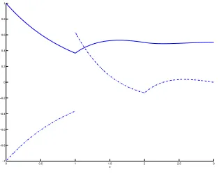
The graphs of u and it’s derivative are plotted in Figure 1. This first representation already sheds some light on the possible behavior of u for atomic Lévy measures: in general u is not monotone, is asymptotically linear at zero, and possibly non-differentiable.
Let us consider the issue of differentiability in more detail. Apparently u is infinitely differentiable in the open intervals(n,n+1), n=0, 1, ..., with
u′(x) =
(
−e−x :x <1,
−e−x +Pni=1(x(i−−i)i−1 1)! e
−(x−i)−Pn
i=1
(x−i)i i! e
0 0.5 1 1.5 2 2.5 3 !1
!0.8 !0.6 !0.4 !0.2 0 0.2 0.4 0.6 0.8 1
x
u(x)
Figure 1:u(solid curve),u′(dashed curve) forδ=1 andΠ =δ1
The only problematic points are the integers at which the piecewise defined function u′gets the additional summands
(
e−(x−1)−(x−1)e−(x−1) :n=1,
(x−n)n−1 (n−1)! e
−(x−n)−(x−n)n
n! e
−(x−n) :n>1,
when going from x<n to x>n. This sheds some light on differentiability as for x=1the right deriva-tive is 1and the left derivative0whereas for n >1the remainder summand vanishes. In particular, this implies that u is differentiable everywhere except at1with
u′(x+)−u′(x−) = Π({x}).
Taking higher order derivatives, the same reasoning shows that at{n}, u is(n−1)-times but not n-times differentiable.
The example reveals three properties which we aim to understand for general subordinators: higher order differentiability ofudepends crucially on the atoms ofΠ,uis generally not monotone andu′
vanishes at infinity and is asymptotically linear at zero.
3
Results
Our Fourier analytic approach forces us to control the small jumps. To this end we recall the Blumenthal-Getoor indexβ(Π)for subordinators:
β(Π) =infnγ >0 :
Z 1
0
xγΠ(d x)<∞o.
Some of our main results are formulated under the following assumption.
Assumption(A). Assume thatβ(Π)<1.
3.1
Series and Integral Representations
The main objective are the potential densities. Our results are motivated by the following extension of the renewal type equation foru.
Lemma 1. The q-potential measure U(q)(d x)has a density u(q)satisfying the renewal type equation
δu(q)(x) =1− Z x
0
u(q)(x−y)(Π(¯ y) +q)d y. (3.1)
Iterating the renewal type equation (3.1), one heuristically obtains a series representation for the potential density u(q). Making this a rigorous statement is slightly involved as ¯Π might have a singularity at zero. The problems caused by the singularity can be circumvented taking into account only the local integrability of ¯Π at zero which is a direct consequence of the property (1.1). In
[CKS10]a proof for the following proposition was carried out for non-atomic Lévy measures. In fact this proposition can be recovered from Chapter 3 in [K72] where it is disguised in terms of
p-functions. For completeness we sketch a proof below.
Proposition 1(Series Representation foru(q)). The series representation
u(q)(x) =
∞
X
n=0 (−1)n
δn+1 1∗ Π +¯ q
∗n
(x) (3.2)
holds for the potential densities u(q). Here,1denotes the Heavyside function.
At this point we should note that for q = 0, Equation (3.2) appears in a slightly different form in [CKS10]. This is due to a different definition of convolutions. In this paper we define the convolution of two real functions f andg by
f ∗g(x) =
Z x
0
f(x−y)g(y)d y,
(and 1∗f∗0(x) = 1) whereas in [CKS10] the convolution was defined by f ∗g(x) = Rx 0 f(x −
y)g′(y)d y. In any case, with F(x) =R0x f(t)d t andG(x) =R0xg(t)d t, we haveF∗G=1∗f ∗g, where the second convolution is in the sense of the present paper.
Unfortunately, deriving properties ofu(q)from (3.2) is a delicate matter as one has to deal with an infinite alternating sum of iterated convolutions. Nevertheless, one particular property that follows from (3.2) is thatu(q)is of bounded variation.
Corollary 1. There are increasing functions u(q)1 and u(q)2 such that
u(q)=u(q)1 −u(q)2 .
To obtain a deeper understanding, we introduce a more carefull representation for u(q) based on Fourier analysis. In the following we denote by
Lf(s) =
Proposition 2(Laplace Inversion Representation ofu(q)). Under Assumption(A), for arbitrary integer N larger than0and any fixedλ >0,
is a well defined absolutely integrable function inθ and
u(q)(x) =
There is a good reason to not only consider the simplest caseN=1. LargerN makes the integrand decay faster which is needed to derive higher order differentiability via interchanging differentiation and integration. ForN>1 it is still easy to work with representation (3.3) as the finite sum can be tackled termwise and for the integral classical convergence results can be applied.
As a first application of Proposition 2 we derive a representation for the first derivative of the po-tential densities. In contrast to Proposition 2 we are not free to chooseN =1; the minimalN now depends on the Blumenthal-Getoor index.
Corollary 2. The right and left derivatives of u(q)exist and are given by
u(q)′
Moreover, under Assumption(A)the following representations hold for N >−β(Π)1−1 andλ >0:
u(q)′
For everyλ >0the function
hN,q(λ+iθ) = − L(Π +¯ q)(λ+iθ)
N
δN+1 1+1
δL(Π +¯ q)(λ+iθ)
Remark 1. We should note that a refinement of the approach of[CKS10]for non-atomic Lévy measures yields the series representation (3.4), (3.5) without assuming Blumenthal-Getoor index smaller than1. Indeed, the difference is that in our settingΠ¯ can have jumps and therefore is outside of the scope of [CKS10]. However, the jumps do not affect the study of the uniform and absolute convergence of the series in(3.4)and(3.5), and it can be carried out as in[CKS10].
The arguments of [CKS10] are not repeated here; we only prove the more usefull Laplace inversion representation under Assumption(A)and derive from this the series representation.
Remark 2. We do not know how to derive the asymptotics of u′ at infinity only from the series rep-resentation (3.4), (3.5). It seems that a reprep-resentation of the type(3.6), (3.7) is much more useful for studying the properties of u′and therefore it is an interesting problem to get such a representation without Assumption(A).
3.2
Higher Order (Non)Differentiability for the Potential Densities
Having established thatu(q)is of bounded variation in Corollary 1,u(q)must be differentiable away from a Lebesgue null set. The null set can be identified as the set of atoms as a consequence of either of the representations given in Corollary 2.
Corollary 3. The potential densities u(q) are differentiable at x if and only if x is not an atom ofΠ. More precisely,
u(q)′
(x+)− u(q)′
(x−) =Π({x})
δ2 . (3.8)
It is interesting to see that the derivative ofu(q)only jumps upwards and how the size of the jumps is determined by the weight of the atoms and the drift. The reader might want to compare this with Figure 1.
Unless explicitly mentioned, from now on we assume that Assumption (A) holds.
The remaining part of this section deals with higher order differentiability properties of the q -potentials. The study focuses on subordinators whose Lévy measure has atoms which accumulate at most at zero. To emphasise the effect of atomic Lévy measure on differentiability, the results are divided into three theorems for non-atomic Lévy measure, purely atomic Lévy measure, and Lévy measure with atomic and absolutely continuous parts.
The case of non-atomic Lévy measure already appeared in[CKS10]. For Blumenthal-Getoor index smaller than 1 their results follow easily from the Laplace inversion representation. To present a complete picture we state and reprove the following result of[CKS10]for smooth Lévy measures.
Theorem 1. IfΠ¯is everywhere infinitely differentiable, then U(q)is everywhere infinitely differentiable.
More accurate effects of the atoms on differentiability are revealed in what follows. The explicit calculation of Example 1 for Π = δ1 indeed suggests more interesting behavior for higher order
n. The critical pointsn∈Nin the example have the property that they can be reached by precisely
njumps of the size of the atom 1.
Denote byGthe atoms of the Lévy measureΠ. We say that x>0 can be reached bynatomic jumps if x=Pni=1gi withgi∈G. Fork≥1 we define the sets
Gk=
¨
x >0 :x =
j X
i=1
gi,gi∈G, 1≤ j≤k
«
of points that can be reached by at mostkatomic jumps. The next theorem shows how higher order differentiability is connected to the setsGk. As it is formulated for purely atomic Lévy measures it can be seen as the counterpart of Theorem 1.
Theorem 2. If Πis purely atomic with a possible accumulation point of atoms only at zero, then, for k≥1,
U(q)is(k+1)-times differentiable at x ⇐⇒ x∈/Gk.
In particular, if x cannot be reached by atomic jumps only, then U(q)is infinitely differentiable at x.
The following example shows that we can easily find examples with exotic differentiability proper-ties.
Example 2. If Πhas atoms on1/k for k≥1, then U(q)is infinitely differentiable at x if and only if x ∈/Q. For x=n/k, U(q)is at most n-times differentiable at x.
Finally, we show how Theorems 1 and 2 combine each other: the atoms prevent U(q) from being twice differentiable and an additional absolutely continuous part does not change the behavior.
Theorem 3. IfΠ(¯ x) =Π¯1(x) +Π¯2(x), whereΠ1 is purely atomic with possible accumulation point of atoms only at zero andΠ¯2 is infinitely differentiable, then, for k≥1,
U(q)is(k+1)-times differentiable at x ⇐⇒ x∈/Gk.
In particular, if x cannot be reached by atomic jumps only, then U(q)is infinitely differentiable at x.
Remark 3. In fact Theorem 3 is still true if Π¯2 possesses only finitely many derivatives. Then the statement will be valid, for any k, such thatΠ¯2is k-times differentiable.
Remark 4. Recalling the close connection of u and creeping probabilities given in (2.1), it would be interesting to have a good probabilistic interpretation of non-existence of derivatives of certain order for the creeping probabilities.
3.3
Asymptotic Properties of Potential Densities
Asymptotic properties at zero and infinity ofU are classical results in potential theory of subordina-tors (see for instance Proposition 1 of Chapter 3 in[B96]). Also the limiting behavior of the renewal densityuat zero and infinity are known (see (2.3) and (2.4)).
In what follows we aim at giving more refined convergence properties based on the representations foru(q) and(u(q))′. Some results will be only valid forq =0. Utilizing the series representation of Section 3.1, we first strengthen the asymptotic at zero. In the following f ∼ g denotes strong asymptotic equivalence, i.e. limf
Theorem 4. For general subordinator with positive drift and n≥ 0, the following strong asymptotic equivalence holds:
n X
k=0 (−1)k
δk+1 1∗(q+Π)¯
∗k(x)−u(q)(x)
∼ (−1) n
δn+2 1∗(q+Π)¯
∗(n+1)(x), as x →0.
The first order asymptotic of (2.3) appears in the theorem for n = 0 and reveals more precise qualitative information:
Corollary 4. The potential density u(q)is asymptotically linear with slope−(Π(R) +q)/δ2 at zero iff the Lévy measure is finite. If the Lévy measure is infinite, then u(q)decays faster than linearly.
A simple class of examples are stable subordinators with drift.
Example 3. If the Lévy measure has stable law withα∈(0, 1), the strong asymptotics at zero are given by
1
δ−u(x)∼
1
δ2C
Z x
0
1
yα d y= C
δ2(1−α)x 1−α.
Lévy measure putting mass precisely to one point provides an example of asymptotically linear behavior.
Example 4. If the Lévy measure has only one atom at 1 and δ = 1, then the direct calculation in Example 1 or Corollary 4 both lead to the linear asymptotics
1−u(x) =1−e−x ∼x, as x →0.
As for absolutely continuous Lévy measures the existence of the derivative of the renewal density was established quite recently, the asymptotics ofu′seem to be unknown. On first view one might be tempted to differentiate the asymptotics of u to derive the asymptotics of u′. Due to lack of knowledge on ultimate monotonicity of uandu′ we cannot apply the monotone density theorem and instead work with the representations of Section 3.1.
Theorem 5. Assume condition(A), i.e. β(Π)<1. LetΠ(¯ 0+) =∞, then there exists n≥1such that
β(Π)≤ n+n1 and then
u(q)′
(x+) =−Π(¯ x+)
δ2 +...+
(−1)nΠ¯∗n(x)
δn+1 +o(1), as x→0,
u(q)′
(x−) =−Π(¯ x−)
δ2 +...+
(−1)nΠ¯∗n(x)
δn+1 +o(1), as x→0.
IfΠ(¯ 0+)<∞then, as x→0,
u(q)′
(x+) =q+Π(¯ x+)
δ2 +o(1),
u(q)′
(x−) =q+Π(¯ x−)
For a large class of processes this implies that the asymptotic of (u(q))′ are indeed given by the derivative of the asymptotic ofu(q):
Corollary 5. If Π has Blumenthal-Getoor index β < 1/2, then u(q)′
(x+) ∼ −q+Π(x¯δ2+) and
u(q)′
(x−)∼ −(q+Π)(x¯δ2 −)at zero.
The hypothesis of the theorem is not necessary to have the asymptotic ¯Π(x)/δ2 at zero as the next example shows.
Example 5. If X is stable with indexα∈(0, 1)and driftδ >0, then
¯
Π∗2(x) =C1
Z x
0
(x− y)−αy−αd y=C2x−2α+1
and inductivelyΠ¯∗n(x) =Cnx−nα+n−1. This, combined with Theorem 5, implies that
u′(x)∼ −Π(¯ x)
δ2 =−
C1x−α
δ2 , as x→0.
Finally, we consider the asymptotics ofu′at infinity which is technically more involved as we could not derive the asymptotics from the series representation (3.4), (3.5). Instead, the proof is based on a refinement of the Laplace inversion representation.
Theorem 6. IfE[X1]<∞, then
lim
x→∞u
′(x+) = lim
x→∞u
′(x−) =0.
As our approach does not work for infinite mean subordinators, it remains open whetheru′vanishes at infinity or not in this setting.
4
Proofs
4.1
Series and Integral Representations
Proof of Lemma 1. When q=0 the statement was already mentioned in Section 2.1 and is due to Kesten (see[K69]). Let us now fixq>0. First note that for any random variableeq∼E x p(q)which is independent ofX using the Markov property at timeeqand integrating out the possible positions
ofXeq ≤x we get
U(x) =E
Z eq
0 1{X
t≤x}d t
+
Z x
0
U(x−y)P(Xeq ∈ d y) =U
(q)(x) +qU∗u(q)(x),
sinceu(q)is continuous and bounded whenever the subordinator possesses a positive drift, see (iii) in Theorem 16 in[B96]. Therefore, differentiation yields
Comparing the latest with
δu(x) =P(XTx =x)
=P(XTx =x;Tx ≤eq) +
Z x
0
P(XT(x−y)=x−y)P(Xeq ∈d y)
=P(XT
x =x;Tx ≤eq) +qδ Z x
0
u(x− y)u(q)(y)d y,
we get the expected relation
P(XT
x =x;Tx ≤eq) =δu (q)(x).
We use this final relation to write
P(Tx ≤eq) =1−P(Xe
q≤ x) =δu
(q)(x) +P(X
Tx > x;Tx ≤eq).
Next we have, using the compensation formula from Chapter 0 in[B96],
P(XT
x >x; Tx ≤eq) =q
Z ∞
0
e−qtE X
s≤t
1{X
s−≤x;Xs>x}
d t
=q
Z ∞
0
e−qt
Z t
0
Z x
0
¯
Π(x−y)P(Xs∈d y)ds
=
Z x
0
¯
Π(x−y)u(q)(y)d y.
This, combined withP(Xe
q ≤x) =q Rx
0 u
(q)(y)d y, proves the assertion.
Proof of Proposition 1: Since ¯Πmay not be continuous, we cannot directly apply the general Theo-rem 6 of[CKS10]. Nonetheless, the proof of Theorem 6 of[CKS10]can be adapted to this situation by noting that in fact it is not crucial that gthere is continuously differentiable but the fact that it is almost everywhere differentiable with a negative derivative vanishing at infinity. The latter is due to the fact that g′is used in convolutions. In this case, for completeness, we sketch a proof but we refer to[CKS10]for details. First note that each summand of
φ(x):=
∞
X
n=0
(−1)n1∗ Π +¯ q
∗n
(x)
δn+1 , (4.1)
is finite as for subordinatorsR1
0 xΠ(d x)is finite showing that ¯Πis not exploding too fast at zero. We
now show that the series is absolutely converging in particular showing that it is well defined and can be rearranged. First, since1∗ Π +¯ q∗(n−1)
(x)is increasing we get iteratively
1∗ Π +¯ q∗n
(x)≤ 1∗ Π +¯ q
(x)n. (4.2)
As1∗(Π +¯ q)(x)is continuously increasing and1∗(Π +¯ q)(0) =0 there is b>0 such that for all
Now we use an iterative procedure to extend the absolute convergence to all x >0: reasoning as
Iterating this arguments as in the proof of Theorem 6 of[CKS10]shows locally uniform and absolute convergence of the series for all x > 0. To verify that φ equalsu we exploit Fubini’s theorem to obtain
implying thatφis a solution of Equation (3.1). Uniqueness of solutions for locally bounded func-tions follows since for two solufunc-tions f andφ
|f −φ|(x)≤ |(f −φ)∗1/δ(Π +¯ q)(x)| as shown above since it is a member of uniformly convergent series.
Proof of Corollary 1. The proof follows directly from Proposition 1. To define the functionsu(q)1 and
u(q)2 we separate the positive and negative parts as
u(q)(x) =
which is possible taking into account the absolute convergence of the series representation. Each summand of the defining series for u(q)1 and u(q)2 is increasing, thus, u(q)1 andu(q)2 themselves are increasing.
Let us first motivate the approach. Taking into account the series representation we divideu(q)into two parts:
u(q)(x) =
N−1
X
n=0 (−1)n
δn+1 1∗ Π +¯ q
∗n
(x) +X
n≥N
(−1)n
δn+1 1∗ Π +¯ q
∗n
(x)
=:
N−1
X
n=0 (−1)n
δn+1 1∗ Π +¯ q
∗n
(x) +φN,q(x).
The goal of the following Fourier analysis is to derive a convenient integral representation forφN,q. For this sake first note that it follows as in the proof of Proposition 1 thatφN,qis the unique locally bounded solution of the following renewal type equation:
φN,q(x) = (−1)
N
δN+1 1∗ Π +¯ q
∗N
(x)− 1
δφ
N,q(x)∗(Π +¯ q)(x). (4.3)
If we were allowed to turn convolution into multiplication in Laplace domain forRe(s)>0, Equation (4.3) transforms into
LφN,q(s) = (−1)
N
δN+1 L1(s)L(Π +¯ q)(s)
N− 1
δLφ
N,q(s)L(Π +¯ q)(s). (4.4)
Solving (4.4) forLφN,q, leads to
LφN,q(s) = (−1)
NL1(s)(L(Π +¯ q)(s))N
δN+1(1+1
δL(Π +¯ q)(s))
=:gN,q(s) (4.5)
whenever the quotient is well-defined. If furthermore we were able to verify integrability conditions needed for Laplace inversion we obtain an integral representation for φN,q. We are now going to
check what is needed to turn this formal approach into rigorous statements.
For the rest of this section we setδ=1in order to simplify the notation.
For the first step it is shown that indeed Equation (4.3) turns into Equation (4.4). A priori this is not clear due to the possible singularity of ¯Πat zero.
Lemma 2. There isλ0≥0such thatLφN,q solves (4.4) on{λ+iθ:λ≥λ
0,θ∈R}.
Proof. To show that the first transformation can be carried out we show fors=λ+iθ,λbounded from below by someλ0, thatL(Π+¯ q)(s)andLφN,q(s)are well defined to deduceL(Π+¯ q)∗n(s) =
L(Π+¯ q)(s)n,L(Π+¯ q)∗φN,q(s) =L(Π+¯ q)(s)LφN,q(s), andL1∗(Π+¯ q)(s) =L1(s)L(Π+¯ q)(s).
To validate Laplace transformation of(Π +¯ q)nforλlarge enough, note that we may chooseλ0such
that
Z ∞
0
which is possible asR01Π(¯ x)d x < ∞and limx→∞Π(¯ x) =0. It now follows directly from Fubini’s
theorem that iterated convolutions of ¯Π +qturn into multiplication under Laplace transforms. We now show thatφN,qcan be Laplace transformed for which we use the fact that
∞
to justify the change of summation and integration in the following:
LφN,q(s) =
The second step in our analysis consists of showing that the convolution Equation (4.4) can indeed be solved in Laplace domain leading to Equation (4.5). The following lemma is stronger then the previous as we can show that gN,q(s)is well defined for anys=λ+iθ withλ >0 even though a priori we do not know thatgN,q is the Laplace transform ofφN,q.
Lemma 3. Suppose thatΠis non-trivial, then gN,q(λ+iθ)is well-defined forλ >0.
Proof. To show thatgN,q(s)is well-defined ats∈Cwith positive real-part, it suffices to show that
L(Π +¯ q)(s)6=−1.
Let us assume thatL(Π+¯ q)(s0) =−1 for somes0=λ0+iθ0withλ0>0. Without loss of generality
way may assumeθ06=0 as otherwise the contradiction follows trivally. The assumption necessarily
Dividing the integral of the absolutely integrable function e−λ0x(Π +¯ q)(x)sin(θ
0x) into pieces of
the length of one period of the sine function and applying Fubini’s theorem, we obtain
0=
Z ∞
0
e−λ0x(Π +¯ q)(x)sin(θ 0x)d x
=
Z ∞
2π/θ0
∞
X
k=0 1[2kπ/θ
0,2(k+1)π/θ0)(x)e
−λ0x(Π +¯ q)(x)sin(θ
0x)d x
=
∞
X
k=0
Z 2(k+1)π θ0
2kπ θ0
e−λ0x(Π +¯ q)(x)sin(θ 0x)d x.
As e−λ0xΠ(¯ x) is strictly decreasing, unless(Π +¯ q)(x) = 0 and (Π +¯ q)(x) is non-increasing each
summand
Z 2(k+1)π θ0
2kπ θ0
e−λ0x(Π +¯ q)(x)sin(θ 0x)d x
must be non-negative and hence vanish as the total sum is zero. In particular, this implies that ¯
Π(x) +q=0 for allx >0 so that forq>0 a direct contradiction occurs. Forq=0 the contradiction occurs asΠwas assumed to be non-trivial. Thusg(s)is well-defined.
Remark 5. If furthermoreE[X1] < ∞, then gN,0 is well-defined also on the imaginary axis. This follows from the same proof noting that in this case (4.9) holds as well forλ0=0. Indeed as each term
R
2(k+1)π θ0 2kπ
θ0
¯
Π(x)sin(θ0x)d x has to vanish we conclude that Πhas to be concentrated on{2kπ/θ0}k≥1.
On the other hand, in this case, as
Re(LΠ(¯ s0)) =
Z ∞
0
e−λ0xcos(θ
0x)Π(¯ x)d x
=X
k≥0
¯
Π2kπ
θ0
Z
2(k+1)π θ0
2kπ θ0
cos(θ0x)d x=0,
we see that Re(LΠ(¯ s0))6=−1and thus gN,q(s)is well-defined.
The third step of our derivation of an integral representation foru(q) is an inversion approach for
gN,q. We now briefly discuss the connection to Fourier transforms which is crucial for the inversion: for integrable functions f define for x ∈R
Ff(x) =
Z ∞
−∞
e−i x tf(t)d t.
Apparently, the Fourier transformF appears when evaluating the Laplace transform on the imagi-nary line only. Defining the auxiliary function
the simple connection is
Frλ(θ) =L(Π +¯ q)(λ+iθ).
Taking into account this close connection of Laplace and Fourier transforms, classical Fourier inver-sion forλ >0 gives the inversion formula (also known as Bromwich integral)
φN,q(x) = 1
2π
Z ∞
−∞
LφN,q(λ+iθ)e(λ+iθ)xdθ
= 1
2πe
λx Z ∞
−∞
gN,q(λ+iθ)eiθxdθ
if gN,q(λ+iθ)is absolutely integrable with respect toθ. To prove the needed integrability we start with a simple estimate.
Lemma 4. For any a>0and y≤ a the estimateΠ(¯ y)≤C(a,ǫ)y−(β(Π)+ε)holds for allǫ >0with
β(Π) +ǫ <1.
Proof. First note that by the definition of the Blumenthal-Getoor indexR01 yβ(Π)+ǫΠ(d y)<∞ for anyǫ >0. The claim follows from the simple observation that for anyα >0 there isδ >0 such that for anyτ < δ
α≥ Z δ
τ
yβ(Π)+ǫΠ(d y)≥τβ(Π)+ǫ(Π(¯ τ)−Π(¯ δ))
as ¯Πis decreasing. Lettingτgo to zero, we deduce lim supτ→0τβ(Π)+ǫΠ(¯ τ)≤α.
The need for Assumption(A)comes from the following lemma and its consequences.
Lemma 5. For anyλ >0andε >0the following estimate holds:
|LΠ(¯ λ+iθ)| ≤ (
C1λ :|θ| ≤1,
C|θ|β(Π)+ε−1 :|θ|>1,
where C=C(ǫ)>0.
estimate forθ >0:
where we have used Lemma 4 and thatrλis decreasing in the last inequality. Unfortunately, this uni-form inλupper bound is not suitable for allθas the constant of Lemma 4 explodes asθ approaches zero. To circumvent this problem we derive a different upper bound that works everywhere equally well but is not uniform inλ:
Similarly, we estimate the real part
The upper bound can now be used to derive the necessary integrability ofgN,q.
Lemma 6. For arbitrary integer N larger than0and anyλ >0we have
Z ∞
Proof. As we have already found a good upper bound forLΠ(¯ s)in the previous lemma, it suffices to show that the denominator
p(λ+iθ) =1+L(Π +¯ q)(λ+iθ)
is bounded away from zero. In Lemma 3 we have shown thatp(λ+iθ)has no zeros forλ≥0 and, hence, by continuity of p it suffices to show that as |θ| tends to infinity p(λ+iθ) stays bounded away from zero. To this end it suffices to note that from Lemma 5
lim
The right hand side is integrable inθ as by assumptionβ(Π)<1 andǫcan be chosen sufficiently small so thatN(β(Π) +ǫ−1)<0.
Proof of Proposition 2: Forλ≥λ0,λ0 satisfying
R∞
0 e
−λ0x(Π +¯ q)(x)d x <1 we can directly follow
the strategy explained before Lemma 2. The proof then follows directly from the definition ofφN,q
and Laplace inversion justified by Lemmas 2, 3, and 6.
The proof of the proposition is complete if we can show that for arbitrary 0< λ < λ0
Z closed contour formed by the pieces
Γ(λ0)∩ {|θ| ≤R},
taken with the right orientation implies the claim. Note that the integrals over the horizontal pieces vanish asRtends to infinity:
lim the integral over ˜Φ(R)vanishes.
Proof of Corollary 2: As remarked after the corollary, the arguments of[CKS10]will not be repeated. Instead, under Assumption (A) we prove the Laplace inversion representation and deduce from this the series representation of[CKS10].
We first show that the right and left derivatives ofu(q)exist and are given by the representation of the theorem. First, right and left derivatives of the finite sum in (3.3) exist by termwise differentiating the finite sum and using that1∗ Π +¯ q∗n
(x) =Rx
0 Π +¯ q
∗n
(y)d y is differentiable from the left and the right with derivative Π +¯ q∗n
(x−) (resp. Π +¯ q∗n
(x+)). As iterated convolutions are continuous, only the first summand is not everywhere differentiable.
To see that the integral is differentiable atx and to deduce the integral representation of(u(q))′note that
The differentiation under the integral is justified by dominated convergence and the upper bound
derived in (4.12) which is integrable inθ for sufficiently smallǫby our choice ofN.
As a second step we now derive the pointwise series representation from the Laplace transform representation of(u(q))′. As for (4.12) we obtain the upper bound
hN,q(λ+iθ)
≤C|LΠ(¯ λ+iθ)|N ≤ (
Cλ1N :|θ| ≤1,
C|θ|N(β(Π)+ǫ−1) :|θ|>1, (4.13)
for arbitrary ǫ >0. To prove the corollary it suffices to show that for N tending to infinity, the Laplace inversion integral
eλx 1
2π
Z ∞
−∞
eiθxhN,q(λ+iθ)dθ
vanishes for fixed x >0 and λ > 0. With our choice ofǫ, i.e. β(Π) +ǫ−1< 0, (4.13) implies pointwise convergenceeiθxhN,q(λ+iθ)→0. We are done if we can justify the change of limit and integration. This comes from the uniform (forN≥2[(β(Π) +ǫ−1)−1] +2 ) inθ integrable upper
bound
eiθxhN,q(λ+iθ) ≤
(
C :|θ| ≤1,
C|θ|−2 :|θ|>1,
and the dominated convergence theorem.
4.2
Higher Order (Non)Differentiability
In this section the results on differentiability are proved. In contrast to Corollary 3, which follows either from differentiating the Laplace inversion representation or differentiating termwise the series representation of u(q), the proofs for higher order derivatives are exclusively based on the more elegant Laplace inversion approach. This forces us to assumeβ(Π)<1 and we do not see how to circumvent this (probably dispensable) restriction.
To reduce the proofs to (non)differentiability of iterated convolutions, differentiability of the Laplace inversion integral is ensured in the next lemma ifNis sufficiently large.
Lemma 7. For N >−β(Π)k−1, the Laplace inversion integral in (3.3) is everywhere k-times continuously differentiable in x with
dk
d xke λx 1
2π
Z ∞
−∞
eiθxgN,q(λ+iθ)dθ= 1
2π
Z ∞
−∞
e(λ+iθ)x(λ+iθ)kgN,q(λ+iθ)dθ.
Proof. To check that we can differentiate
eλx 1
2π
Z ∞
−∞
eiθxgN,q(λ+iθ)dθ
k-times under the integral, by dominated convergence we need to find an integrable upper bound for the derivative:
dk
d xke
iθxgN,q(λ+iθ) =
θ
Integrability follows directly from the choice ofN and the integrable upper bound (4.12) for suffi-ciently smallǫ.
Having understood differentiability of the remainder term, to prove higher order differentiability of
u(q) we choose N large enough to apply the previous lemma and then deal with the finite sum of convolutions. Here is a lemma for smooth Lévy measures.
Lemma 8. If f : R → R+ with f(x) = 0 for x ≤ 0 is infinitely differentiable on R+ and locally integrable at zero, then f∗nis everywhere infinitely differentiable and integrable at zero for any n≥1.
Proof. The proof is easily conducted by induction with basis n = 1, i.e. f(x). Then the simple identity
f∗(n+1)(x) =
Z x
2
0
f∗n(x−y)f(y)d y+
Z x
2
0
f∗n(y)f(x−y)d y
and the induction hypothesis confirm the statement of the lemma with respect to differentiability. The integrability follows similarly from the representation
Z 1
0
f∗(n+1)(x)d x=
Z 1
0
f∗n(y)
Z 1−y
0
f(s)dsd y
and the integrability of f(x)at zero.
Combining the previous lemmas we can prove Theorem 1.
Proof of Theorem 1: As the potential measure U(q) is differentiable with derivativeu(q), to differ-entiate (k+1)-times U(q) it suffices to differentiate k-times the potential density u(q). Applying Proposition 2 withN>− k
β(Π)−1 yields
dk+1
d xk+1U
(q)(x) = d k
d xku (q)(x)
= d
k
d xk N−1
X
n=1 (−1)n
δn+1 1∗(Π +¯ q)
∗n(x) + d
k
d xke λx 1
2π
Z ∞
−∞
eiθxgN,q(λ+iθ)dθ.
AsN was assumed to be large enough, the integral is everywherek-times differentiable by Lemma 7. Forβ(Π)close to 1 the sum might be arbitrarily large but is always finite. So we can differentiate termwise the sum and use d
d x1∗(Π +¯ q)
∗n(x) = (Π +¯ q)∗n(x)as ¯Πis continuous leading to
dk+1
d xk+1U
(q)(x) = N−1
X
n=1 (−1)n
δn+1
dk−1
d xk−1(
¯
Π +q)∗n(x) +eλx 1
2π
Z ∞
−∞
eiθx(λ+iθ)kgN,q(λ+iθ)dθ.
(4.14)
The proof revealed the full strength of the Laplace inversion approach compared to the series ap-proach of [CKS10]. Their major technical problems consist of justifying differentiation under the alternating infinite sum (3.2). As we split the infinite sum into a harmless finite sum and an integral which can be dealt with easily, the main problems of[CKS10]have been circumvented.
Next we analyze the influence of atoms of Π on (non)differentiability for which we start with a lemma on higher order convolutions for discrete Lévy measures.
Lemma 9. SupposeΠis purely atomic with possible accumulation point of atoms only at zero, then
(a) Π¯∗nis a polynomial of order at most n−1away from G
nfor n≥1,
(b) Π¯∗nis everywhere(n−2)-times differentiable but not(n−1)-times differentiable at Gn\Gn−1for n≥2.
Proof. The proof is based on the simple observation
1[0,a]∗f(x) =
(Rx
x−af(y)d y :a< x, Rx
0 f(y)d y :a≥ x,
(4.15)
for integrable f vanishing on the negative half-line. Hence,1[0,a]∗f is continuous everywhere and differentiable atx and x+a if and only if f is continuous at x. We will resort to the fact that asΠ
is purely atomic, ¯Π = Π(x,∞)is piecewise constant and can be represented as linear combination of step functions, i.e.
¯
Π(x) =X
a∈G
Π({a})1[0,a](x). (4.16)
To prove (a) we proceed by induction which we start with n = 1. Taking into account (4.16), ¯
Π∗1 =Π¯ is a polynomial of order 0 away fromG. Next, assume that ¯Π∗n is a polynomial of order
at most n−1 away from Gn. To prove the claim for ¯Π∗(n+1), we fix an interval (d,b) such that
d ∈Gn+1∪ {0}, b∈Gn+1 and(d,b)∩Gn+1=;. Our aim is to show that for everyx ∈(d,b)there is an open interval∆(x)⊂(d,b) such that ¯Π∗(n+1)is polynomial of order at most non∆(x). Fix
x ∈(d,b)and choosea∗(x) =max
c∈G∪ {0} : x−c>d . As the atoms accumulate only at zero there is a neighbourhood∆(x) ofx such that z−a∗(x)>d for everyz ∈∆(x). Next, by Fubini’s theorem we observe
¯
Π∗(n+1)(x) =X
a∈G
Π({a})1[0,a]∗Π¯∗n(x). (4.17)
By the induction hypothesis and (4.15) all summands are locally polynomials of order at most n. To show that ¯Π∗(n+1)is a polynomial of order at mostn, we split ¯Π∗n according to the two cases of
(4.15):
¯
Π∗(n+1)(x) = X
x≤a∈G
Π({a})1[0,a]∗Π¯∗n(x) + X
x>a∈G
Π({a})1[0,a]∗Π¯∗n(x)
=
Z x
0
¯
Π∗n(y)d y X
x≤a∈G
Π({a}) + X
x>a∈G
Π({a})
Z x
x−a
¯
The first summand clearly is a polynomial of order at most non ∆(x) by the induction hypothesis
We clearly deduce by the induction hypothesis that the second sum, having finitely many summands only, is a polynomial of order at most n on ∆(x). By the definition of a∗(x) and the induction
the first sum is clearly absolutely summable and henceforth it defines a polynomial of order at most n. Thus we conclude that on∆(x) we have that ¯Π∗(n+1)is a polynomial of order at most n. Representing(b,d) as a union of neighbourhoods∆(x)shows that ¯Π∗(n+1)is indeed a polynomial of order at mostnon(b,d).
In particular, (a) shows that ¯Π∗nis infinitely differentiable away fromGn. To prove the claimed non-differentiability in (b), a different approach is needed. We prove the assertion again by induction in n. The first step is to show that ¯Π∗2 is everywhere continuous and not differentiable at G2\G.
Continuity follows from the continuity of1[0,a]∗Π(¯ x)and the locally uniform convergence of (4.17)
which can, applying monotonicity of ¯Πand the properties ofΠ, be seen forǫsmall enough and N
large enough from
whereC(x)are locally bounded constants.
Now we show that ¯Π∗2 is not differentiable at G
2\G. Although we already know that ¯Π∗2 is a
polynomial away from G2, we derive a second representation showing that for x ∈/ G2 it can be differentiated termwise. As the atoms are discrete, there is a largest atom c < x implying that
we see that1[0,a]∗Π¯ is infinitely differentiable away fromG2. To show that the infinite sum (4.17) can be differentiated termwise forn=1, we derive a locally absolutely and uniformly summable in
x upper bound for the series of derivatives:
X
The first summand is bounded as ¯Π is locally constant. For the second, the sum only runs over
x −c < a as otherwise ¯Π(x)−Π(¯ x−a) = 0. There is no accumulation point of atoms at x, so
Since b ∈ G2\G and G has a possible accumulation point only at zero, the last sum has a finite
number of summands and is strictly positive. The exchange of limit and summation is possible since for all y and x sufficiently close to band alla∈G, such that a<c, for somec >0, y−a∈A(b)
To show that at the critical points ¯Π∗(n+1)is everywhere(n−1)-times differentiable we again verify termwise the differentiability:
d,x)∩Gn =;andd< x becauseG has a possible accumulation point only at zero. The latter also implies that there are at most finitely many atomsasuch that x >a≥d and therefore we need to study only duction hypothesis that ¯Π∗n is (n−2)-times continuously differentiable everywhere. In total we conclude that ¯Π∗(n+1)is(n−1)-times continuously differentiable everywhere.
Finally our task is to show that forb∈Gn+1\Gn
above imply that we can differentiate termwisen-times (4.17) onA(b)\bto get
dn
Using (4.15) we rewrite the latter as
Since b∈Gn+1\Gn we have that either b−a6∈Gn or b−a∈Gn\Gn−1, where the latter is possible only for finitely many, but more than zero, a ∈ G. We mention that the interchange of limit and summation is valid since for allx and y sufficiently close tob, there isc>0, such that for alla∈G
such thata < c, x−a∈A(b)and y −a∈A(b). We have already argued above that the n−1-st derivative of ¯Π∗n is a constant onA(b)due to Lemma 9. By the induction hypothesis for thosea
dn−1
d xn−1Π¯
∗n((b−a)+)− d
n−1
d xn−1Π¯
∗n((b−a)−)>0.
Thus we conclude the induction and the proof of the lemma.
The observation of the lemma motivates the strategy for the main proofs: first, choose N large enough that the integral of the Laplace inversion representation can be differentiated as often as needed. Secondly, consider the finite sum of iterated convolutions for which critical points for kth derivatives only occur for the kth summand. Lower order convolutions vanish and higher order convolutions are smooth enough.
Before we give the main proofs, one more lemma is needed to show how to separate ¯Πandqand afterwards absolutely continuous and discrete part of the Lévy measure.
Lemma 10. SupposeΠis purely atomic with possible accumulation point only at zero. If f is infinitely differentiable away from Gi with locally bounded derivatives and integrable at zero, then Π¯ ∗ f is infinitely differentiable away from Gi+1 with locally bounded derivatives.
Proof. First note that by (4.15) for arbitrarya>0
dk
d xk1[0,a]∗f(x) = ( dk−1
d xk−1f(x)−
dk−1
d xk−1f(x−a) :a<x,
dk−1
d xk−1f(x) :a≥x,
(4.19)
From this simple identity the claim follows for the special caseΠ =δa. For infinitely many atoms
the difficulty appears from the fact that ¯Πis an infinite sum of indicator functions so that summation and differentiation in
¯
Π∗f(x) = X
a∈G
Π({a})1[0,a]
!
∗f(x) =X
a∈G
Π({a})1[0,a]∗f(x) (4.20)
need to be interchanged. To justify the Fubini flip in (4.20) it suffices to show locally uniform absolute convergence of the right hand side. An upper bound can be obtained as
X
x>a∈G
Π({a})
Z x
x−a
|f(y)|d y+ X
x≤a∈G
Π({a})
Z x
0
|f(y)|d y
≤ sup
y∈[x−c,x]
|f(y)| X x>a∈G
Π({a})a+
Z x
0
|f(y)|d y X
x≤a∈G
Π({a}),
zero.
Having justified (4.20), we now show that away fromGi+1
dk
which we prove by showing locally uniform absolute convergence of the series of derivatives. First note that asx ∈/Gi+1there isc′>0 such that(x−c′,x+c′)∩Gi+1=∅. As the setB={a∈G:a>c′}
which again is bounded by property (1.1) and local boundedness of derivatives of f. This is enought to show (4.21) asBis a finite set.
In total we proved that ¯Π∗f is infinitely differentiable away fromGi+1and derivatives may be taken
termwise. Local boundedness of the derivatives follows from the above estimate.
With the lemmas in mind we can give the proofs of the main results.
Proof of Theorem 2. To prove higher order (non)differentiability, we consider the Laplace inversion representation of Proposition 2 forN>−β(Π)k−1:
AsN was assumed to be large enough, the integral is everywherek-times differentiable by Lemma 7 so that the critical points claimed in the theorem have to come from differentiating the finite (possibly very large) sum. As motivated before the proof, N can be chosen arbitrarily large as the higher order convolutions are smooth enough.
Since representation (4.22) is valid replacingk by some n≤ k, we proceed by induction showing thatu(q)isk-times differentiable in x iff x 6∈Gk. The induction basis forn=1 is true in complete generality (without Assumption (A)) due to Corollary 3. Assume next that the claim is true for some
n < k and consider (4.22) with k replaced by n+1. Since the nth derivative does not exist on
Gn, we only need to consider the(n+1)st derivative onR+\Gn. The integral term is(n+1)-times differentiable as seen above so that we only consider the sum