Directory UMM :Journals:Journal Of Public Economics:Vol79.Issue1.Jan2001:

(1)

www.elsevier.nl / locate / econbase

Bequest motives: a comparison of Sweden and the

United States

a b ,_*

John Laitner , Henry Ohlsson a

Department of Economics, University of Michigan, Ann Arbor, MI 48109, USA

b

¨ ¨

Department of Economics, Goteborg University, Box 640, SE-405 30 Goteborg, Sweden

Received 30 July 1998; received in revised form 30 October 1999; accepted 1 November 1999

Abstract

This paper reviews four well-known theoretical models of private bequest behavior, notes their differing implications for public policy, and discusses a way of empirically dis-criminating among them. Then it implements the test with micro data from Sweden (LLS) and the U.S. (PSID). The so-called altruistic (or dynastic) model, which, among the four models, has perhaps the most wide-ranging implications for policy, receives some support. The sign pattern is as the model predicts, while the magnitude is much smaller than the altruistic theory implies. There is evidence of a potential complication due to a dependence of children’s education on parents’ financial status in the case of the U.S.  2001 Elsevier Science B.V. All rights reserved.

Keywords: Accidental model; Altruistic model; Egoistic model; Exchange model

JEL classification: D64; D91

1. Introduction

Bequests and inheritances are potentially important from the viewpoint of public policy. Equality is one issue: the unevenness of inheritances may increase the inequality of society’s distribution of wealth, and the option of leaving an estate may increase inequality of utility among benefactors and among beneficiaries.

*Corresponding author. Tel.:146-31-773-1362; fax:146-31-773-1326. E-mail address: henry.ohlsson@economics.gu.se (H. Ohlsson).

(2)

Efficiency is another consideration. From the standpoint of efficiency, taxation of intergenerational transfers may be desirable since strategic behavior on the part of heirs may be socially wasteful, and inheritances may damp the work incentives of otherwise productive people. Moreover, one theoretical model suggests that bequests are unintentional and might be a source of tax revenue with no corresponding deadweight loss.

Models with intentional bequests lead to more complications. Saving to create estates may be an important source of capital in a market economy, a source which heavy taxation might jeopardize (recall Kotlikoff and Summers, 1981). In addition to financing human capital acquisition on the part of children and grandchildren (e.g., Becker and Tomes, 1979), family line transfers may provide startup capital for entrepreneurs (e.g., Holtz-Eakin et al., 1994; Lindh and Ohlsson, 1996; Blanchflower and Oswald, 1998). In so-called altruistic models, private transfers provide insurance — with bequests tending to flow from more to less prosperous members of family lines — which markets or public authorities may be unable economically to match because of moral hazard. In so-called exchange models, private intergenerational transfers may constitute payments for personal services rendered between members of a family line, and there may be no close substitutes for these services in impersonal markets or public programs. Bequest taxes may, of course, reduce the work incentives of potential donors as well.

Bequest behavior could have implications more generally for public policy. In Barro’s (1974) well-known analysis of the altruistic model, intergenerational transfers within dynastic family lines generate an essentially perfectly elastic supply of private wealth. The effects of public policies such as deficit spending and unfunded social security are completely ‘neutralized.’ Policies, such as switches from income to consumption taxation, designed to increase life-cycle saving may become irrelevant. Taxation of the return to capital, on the other hand, should, in this framework, be avoided (e.g., Chamley, 1986; Lucas, 1990; Ihori, 1997).

Since different models of bequest behavior lead to quite different conclusions about public policy, it is desirable to develop an empirical basis for assessing the validity of competing theories. It seems fair to say that work to date has yielded ambiguous results, sometimes seeming to support one theoretical model and

1

sometimes others. The purpose of the present paper is to provide additional empirical evidence.

We begin with a summary of four contrasting theories, paying special attention to testable differences among them, and considering their implications for taxation.

1

(3)

This is the topic of Section 2. Section 3 describes our data, which consists of panels for Sweden and the U.S. Section 4 tests the different models on each data

2 set. Section 5 concludes.

Parents intentionally, and unintentionally, make transfers to their descendants in a number of ways, including (i) biological transfers of natural talents and abilities, (ii) purchases of education and other human capital, (iii) inter vivos gifts, and (iv) post-mortem bequests of tangible and financial property. Solon (1992) analyzes the relation between incomes of fathers and sons for the U.S. In his regression of log permanent income of sons on log permanent income of fathers, he finds coefficients in the range 0.4–0.5, illustrating the potential importance of biological

¨ ¨

transfers. Using a similar methodology, Bjorklund and Jantti (1997) compare Sweden and the U.S. Although their point estimates of intergenerational correla-tions are lower for Sweden, they fail to reject the null hypothesis that coefficients in the two countries are the same. Recent work by Altonji et al. (1997) studies inter vivos transfers in the U.S. Signs of estimated coefficients are consistent with the altruistic model, but their magnitudes are far smaller than its theoretical predictions.

The present paper considers the fourth channel. As all theoretical models would imply, we find that higher parental resources lead to larger intergenerational transfers. Turning to the problem of discriminating among theories, we uncover some support for the altruistic or dynastic model of bequest behavior in terms of coefficient signs. However, as in Altonji et al. (1997), the magnitudes of our coefficient estimates fall a good deal short of what the model requires. Somewhat surprisingly, similar outcomes emerge from both the Swedish and the U.S. data.

2. Theoretical models

The existing literature suggests a number of possible theoretical models of bequest behavior. This section reviews four of the most prominent. As the Introduction indicates, different models can have quite different implications for public policy.

In one model, an extension of the well-known life-cycle framework, bequests arise accidently (e.g., Davies, 1981; Friedman and Warshawsky, 1990). If adverse selection impedes effective functioning of markets for annuities, households may self-insure against very long life. Then when a household dies young, its unused resources become an accidental bequest. (Or, if it lives a long time, it may die with little or no estate.) Government could heavily tax estates in this case without generating deadweight losses.

2

(4)

In other models, bequests are voluntary. Below we examine three formulations in this vein: the altruistic model, the egoistic model, and the exchange model.

Before doing so, there are important qualifications to make. First, our simple formulations assume that the decisions of those making intergenerational transfers (parents) do not affect the behavior of those receiving transfers (children). Hence, we rule out strategic interactions between donors and donees (cf. Cremer and Pestieau, 1996). Second, we assume price inelastic labor supply for donors and donees (e.g., Holtz-Eakin et al., 1993; Lindh and Ohlsson, 1996). Third, recent data suggest that intergenerational transfers from parents to children are roughly an order of magnitude larger than transfers in the reverse direction (e.g., Kurz, 1984; Gale and Scholz, 1994), and we not study two-sided altruism or transfers from children to elderly parents (cf. Laitner, 1988). Fourth, taxes or liquidity constraints might lead parents to carry out their intergenerational transfer plans prior to their death (e.g., Altonji et al., 1997; McGarry, 1998; Poterba, 1998; Hochguertel and Ohlsson, 1999, and others). Indeed, empirical evidence suggests that inter vivos transfers are substantial (i.e., Gale and Scholz, 1994). Nevertheless, our data and analysis are restricted to bequests and inheritances.

2.1. The altruistic model

In a so-called altruistic model a parent household cares not only about its own lifetime consumption but also about the consumption of its descendants. This is the framework of Becker (1974) and Barro (1974).

Consider a parent who lives one period, period 1, and raises a single child. After period 1, the child is grown and forms a household of its own, the latter lasting

p

one period, period 2. The parent’s total earnings, Y , arrive, of course, in period 1; c

the child’s, Y , arrive in period 2. Both earnings figures are known with certainty p

at time 1. The parent receives inheritance I at the start of period 1 (i.e., as it

p c

receives Y ). One period later the parent provides inheritance I to the child. For simplicity, the interest rate (in this section) is 0.

In the altruistic model, the parent cares about its own period-1 consumption and about its child’s consumption possibilities — hence, about the child’s total

c c

resources Y 1I . We will think of the parent as solving

p p c c c

maxhU(Y 1I 2I )1l ?V(Y 1I )j, (1)

c

I

c

subject to: I $0. (2)

The nonnegativity constraint arises because we assume that parents cannot compel their children to support them. Assume as well that U(.) and V(.) are concave and increasing with U9(0)5 ` 5V9(0). The price of consumption is 1. Parental

p p p c

lifetime consumption is C 5Y 1I 2I , and parental saving for bequests is

p p p

(5)

V(.) measures parental utility from the child’s consumption, and lis a parameter registering the strength of the parent’s altruistic sentiments. Despite the simplicity

3 of (1) and (2), its behavioral implications seem quite general.

p p c

* *

Let T 5T (Y 1I ,Y ,l) be the utility-maximizing transfer to the child in the c

absence of constraint (2), so that I simultaneously solving (1) and (2) is

c p p c

*

I 5maxh0,T (Y 1I ,Y ,l)j. (3)

*

For the latent transfer T , first-order conditions of utility maximization yield

* * *

≠T ≠T ≠T

]]p .0, ]]c ,0, ]]_≠l .0. (4)

≠Y ≠Y

In other words, higher earnings for the parent lead to a higher desired uncon-strained transfer, higher earnings for the child lead to a lower desired transfer, and higher altruism leads to a larger desired transfer. Households could differ in their l’s as well as in their earnings.

p c

*

Notice that having solved (1) for T , if we increase Y by $1 and decrease Y *

by the same amount, raising T by $1 leaves first-order conditions of (uncon-strained) utility maximization satisfied; so

* *

≠T ≠T

]]p 2]]c 51. (5)

≠Y ≠Y

Altonji et al. (1997) employ this condition. Although data limitations force us to concentrate much of our analysis on the sign implications from (4), the U.S. data enable us to consider (5) as well. Two factors worth noting are (i) that actual p transfers include inter vivos gifts as well as post-mortem bequests and (ii) that Y

c

and Y must both be present values with the same base years for (5) to hold in theory. The latter is not a problem when the interest rate is 0, of course. On the former point, Becker and Tomes (1979) stress parents’ role in financing children’s education, and recent work emphasizes the magnitude and importance of inter

*

vivos gifts. Since our empirical analysis of T (.) relies on measured inheritances alone — possibly only one component of each household’s overall intergeneration-al transfer — intergeneration-all of our estimated coefficients may be understatements, perhaps tending to lead us erroneously to reject (5).

Another potential problem is that government student loans, public schooling (including public universities), and scholarships may be insufficient to guarantee that children receive efficient levels of education in the absence of parental

c

generosity. Then Y may be positively correlated withl because both connect to c

*

the child’s education, tending to bias our estimates of≠T /≠Y below. Assuming

3

(6)

that children do manage to obtain efficient amounts of education but that altruistic parents pay the direct costs through transfers which they view as a higher priority than post-mortem bequests, we estimate

c p p c E c

*

I 5maxh0,T (Y 1I ,Y ,l)2P ?E j (6)

c E

below as well as (3). In (6), E is the child’s education, and P is the private cost of units of education.

Although taxing transfers will distort private behavior in the altruistic model, 4

such taxes may promote equality of consumption opportunities. Bequests tend to compensate children for low earnings, and they may do so with fewer problems from imperfect information and moral hazard than public transfers face. However, a parent with extraordinarily high earnings may ‘compensate’ his child with a large estate, but the child, while doing less well than his parent, may still earn more than most others in his generation.

2.2. The egoistic model

In another model which the literature frequently employs (e.g., Blinder, 1974; Hurd, 1989, and others), a parent derives utility from the amount he bequeaths rather than from the amount his child can actually consume. This is sometimes called the egoistic model. Problem (1) and (2) becomes

p p c c

maxhU(Y 1I 2I )1l ?V(I )j, (7)

c

I

*

subject to (2). Looking at the latent variable T maximizing (6) alone, first-order conditions yield

* * *

≠T ≠T ≠T

]]p .0, ]]c 50, ]]_≠l .0. (8)

≠Y ≠Y

Again, (3) characterizes the actual inheritance the child receives. In contrast to the c

altruistic case, an heir’s earnings have no bearing on I .

The overall public policy implications of the egoistic model are quite different from the altruistic case. In particular, Barro’s (1974) famous Ricardian equiva-lency results do not hold. The excess burden from taxing transfers is not clear. If the spirit of the model is that the donor evaluates a transfer solely in terms of his own sacrifice in making it, the argument of V(.) in (7) should be the gross-of-tax transfer, and taxes will not affect the donor’s behavior. If, on the other hand, the donor cares about the absolute amount his heir receives, the argument of V(.) should be the net-of-tax transfer, and there will be a deadweight loss from estate or inheritance taxes.

4

(7)

2.3. The exchange model

Bernheim et al. (1985) and Cox (1987) present versions of the exchange model. In the exchange model, a parent is not altruistic in the sense of caring about the consumption possibilities of his child. Instead, a parent values attention from his child more than services purchased in anonymous markets, and the parent obtains

s

more such attention by making a larger bequest. Let C be the quantity of attention (i.e., services) the parent ‘purchases’ from his child, and let P be the ‘price’ the parent has to pay per unit of the latter. Assuming the child’s time, hence the cost

c

to the child of providing attention, is increasing in Y , we have

≠P c

]

P5P(Y )$0, c.0. (9)

≠Y

Assume the parent solves

p p c s s

maxhU(Y 1I 2P(Y )?C )1l ?V(C )j, (11)

s

C

s

subject to: C $0, (11)

where V(.) measures the parent’s pleasure from the attention of his child. s

‘Inheritance’ amounts in data are to be interpreted as payments for C — in other words

c s c

* * *

T 5P(Y )?C and I 5maxh0,T j, (12)

s *

where C solves (10) without (11).

s p

*

Assuming U(.) and V(.) are increasing and concave, C is increasing in Y ,

c c

decreasing in Y , and increasing inl. The effect of increasing Y on the desired transfer is ambiguous, however, because of the multiplicative role of P(.) in (12). We have

* * *

≠T ≠T ≠T

]]p .0, ]]c . or ,0, ]]_≠l .0. (13)

≠Y ≠Y

(8)

Table 1

Theoretical determinants of bequests and excess burden of taxation Model Parent’s Child’s Excess burden

resources earnings of taxation

Accidental model 1 0 No

Altruistic model 1 2 Yes

Egoistic model 1 0 Yes, if amount received matters No, if amount given matters

Exchange model 1 ? Yes

2.4. Summing up

Table 1 summarizes the implications of the different bequest models. The models share the prediction that more resources for the parent will increase his bequest. On the other hand, they differ on their predictions of how a child’s earnings affect the bequest, and that provides a way for our empirical analysis to shed light on the question of which model is most consistent with data.

3. Sweden and the U.S.

We have data from two quite different industrialized countries, Sweden and the United States. In each case, we have panel data, allowing us to determine households’ lifetime earnings more accurately than would be possible from a single year’s cross section. The data include cumulative inheritances, extensive demographic information, and information about parents.

Before turning to the data, note three potentially important differences between our two countries. First, although both have high standards of living, the government sector in Sweden is a considerably larger fraction of the economy. More generous provision of public goods, services, and transfers, and a more onerous tax system, presumably reduce household incentives in Sweden to arrange private insurance (including insuring descendants’ living standards through private intergenerational transfers). Second, existing research hints that there is less direct transmission of earning ability in Sweden. As stated in the Introduction, Solon (1992) finds coefficients of 0.4–0.5 when he regresses the (log) permanent income

¨ ¨

(9)

of separate inheritances. Swedish tax rates are progressive, and tax liabilities begin 5

at lower levels than is the case in the U.S.

3.1. Swedish data

Our Swedish data comes from the Level of Livings Survey (LLS) collected by the Institute for Social Research at Stockholm University. The LLS consists of a panel running through 1968, 1974, 1981, and 1991. As the 1991 survey omitted questions about inheritances, we employ only the first three waves. Appendix A provides details of the survey questions which we use (see also Laitner and Ohlsson, 1997).

As Appendix A shows, the LLS measures cumulative inheritance by individual in 1968, 1974, and 1981. Later inheritance figures should include earlier amounts plus increments; thus, an individual’s responses should be monotone nondecreas-ing through time. Similarly, the date for an individual’s largest inheritance should never decline. While the general intertemporal consistency of responses seems quite high, we attempt to eliminate deviant reports. Our underlying assumption is that information remembered for the shortest time is the most accurate. For example, if a respondent in 1968 lists the year of his largest inheritance as 1936 but remembers 1938 in 1974, we set both dates to 1936. As we are interested in complete inheritances, we limit our sample to respondents both of whose parents are deceased. To limit the role of life insurance settlements for orphans, we drop respondents of age less than 30. We exclude widows and widowers because they might count funds from their spouses’ estates as inheritances, whereas our analysis applies to intergenerational transfers.

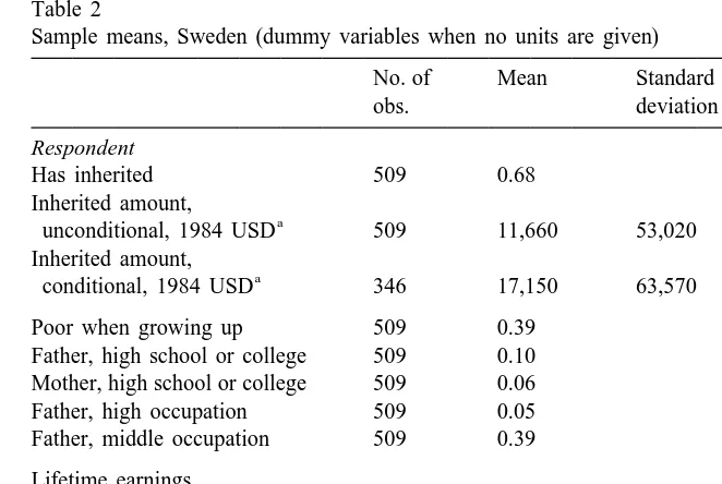
Table 2 shows that over two-thirds of our remaining Swedish individuals have inheritances. A few respondents report having received an inheritance but fail to provide an amount. Our maximum likelihood estimation below incorporates these cases as right-censured data, and we use our estimated coefficients from column 2 of Table 4 to predict the inheritances of these individuals for Table 2. This is not an important issue for Table 2, where we have only four such respondents in column 2, for instance, but it is more significant for the U.S. data which we consider in the next section.

We deflate inheritance amounts to 1984 SEK using the Swedish CPI, then divide by the 1984 PPP exchange rate of 7.71 to convert to U.S. dollars, and finally calculate the present value of an individual’s total inheritance at age 50, assuming a 3% real interest rate. As stated, each wave of the LLS provides one

5

In Sweden, there is an exemption from paying inheritance taxes for each child. This amount corresponded to USD 3300 in 1981 for children aged 18 or more. For younger children there was an additional exemption of USD 700 for each year below 18. The tax rate in the first bracket, taxable amounts ,6500, was 5% in 1981. The highest tax rate was 65%; it applied for taxable amounts

(10)

Table 2

Sample means, Sweden (dummy variables when no units are given) No. of Mean Standard

unconditional, 1984 USD 509 11,660 53,020 Inherited amount,

a

conditional, 1984 USD 346 17,150 63,570 Poor when growing up 509 0.39

Father, high school or college 509 0.10 Mother, high school or college 509 0.06 Father, high occupation 509 0.05 Father, middle occupation 509 0.39 Lifetime earnings,

b

net of taxes, 1984 USD 509 384,030 125,870

Number of siblings 509 4.09 2.87

Age, years 509 63.2 8.95

Woman 509 0.38

Married 509 0.79

Years of education 509 8.79 3.11

a

Includes predictions from column 2, Table 4, for censured values — see text. Inheritance amounts in present value for respondent age 50.

b

Includes hours adjustment on part-time earnings — see text.

cumulative inheritance amount for the respondent and a year of receipt for the 6

largest component in the amount. In deflation and present value calculations, we treat the entire 1968 amount as arriving at the year of its largest component. If the 1974 cumulative amount is larger, we treat the increment over 1968 as arriving at the date provided in 1974 — or 1971 if the new date of receipt is the same as the old one. We repeat this step for 1981.

Table 2 shows that the average inherited amount for our Swedish sample is $11–12,000, and the average amount for those with a positive inheritance is about $17,000.

Our models require measures of an heir’s lifetime earnings (which correspond to c

Y of Section 2). Using LLS panel data on respondents and their spouses, we estimate a standard earnings dynamics equation (e.g., Ahlroth et al., 1997). We convert nominal figures to 1984 dollars as above. For individual i and date t, our regression’s error term is ui1e with u a random individual effect and e iid. Weit i it

run separate regressions for men and women. We use all observations in the original data set with positive earnings (i.e., even respondents with living parents, respondents who are widows, etc.). Employing observations on each individual in

6

(11)

this paper’s sample to derive a conditional estimate of his / her u , we project thei

individual’s earnings at every age to 65 from the maximum of schooling years plus 6 and 16. As we have observations from at most three years, we assume earnings growth mimics GDP per capita at other dates. Using a 3% per year real interest rate, we discount the individual’s lifetime earnings to the year that individual is age 50. We exclude individuals for whom we do not have at least one earnings observation.

We want to value each individual’s time endowment. The LLS provides an annual earnings figure and an average wage rate. Our primary earnings observation is the maximum of the annual earnings figure and 1750 times the average wage. Our adjustment may alleviate endogeneity problems stemming from the possibility that people expecting large inheritances might work fewer hours. For comparison, we derive separate earnings figures with no hours adjustment. Before computing lifetime present values in either case, we subtract local and national income taxes from individuals’ imputed yearly earnings. The tax corrections reflect statutory rates. After-tax figures are compatible with inheritance data.

Table 2 shows that mean net-of-tax Swedish lifetime earnings in present value at age 50 are about USD 384,000 for our sample with adjusted work hours. Clearly the individuals in our sample are quite old on average because of our requirement that their parents be deceased, and this leads to lower lifetime earnings than would otherwise be the case.

Unfortunately, we lack direct observations of the lifetime earnings and inheritance of respondents’ parents. At this point, we use instead a set of five proxies: dummies for whether the respondent reports being poor when growing up, for whether the respondent’s father belonged to a ‘high’ occupational group (i.e., professional or managerial), for whether the respondent’s father belonged to a middle occupational group (i.e., sales, self-employed, clerical, craftsman, or farmer), whether the respondent’s father had a high school education or more, and

7

whether the respondent’s mother had a high school education or more. Table 2 provides sample means for all variables.

Our remaining variables are demographic: number of siblings for the respon-dent, age of the responrespon-dent, whether the respondent is a woman, and whether the respondent is married.

3.2. U.S. data

Our U.S. data comes from the Panel Study of Income Dynamics (PSID). The PSID consists of a random sample (i.e., the ‘SRC sample’) and a special sample of

8

low-income households (i.e., the ‘Census’ or ‘poverty sample’). We provide both

7

The residual occupational categories for the father are operative and laborer. See Table 5 in Juhn et al. (1993) for information on earnings within different categories.

8

(12)

unweighted and weighted regressions below (using 1984 PSID family weights). The weights deemphasize the Census sample, providing a more accurate depiction of the U.S. economy as a whole, and a closer parallel to the Swedish data. Appendix A provides details on the variables we employ.

In 1984 the PSID collected information on cumulative inheritances, including amounts and year of arrival for two. We convert amounts to 1984 dollars using the NIPA consumption deflator, and then, using a 3% real interest rate, deduce the present value of cumulative inheritances in the year the household head was age 50.

One difference from the LLS is that the PSID makes special efforts to elicit data from reluctant respondents. Thus, the PSID routes respondents who say they have received an inheritance but do not recall the amount to a series of brackets, i.e. was the amount over (under) $10,000? over (under) $100,000? or over (under) $1000? Also, the PSID asks respondents if they anticipate receiving an additional inheritance in the next 10 years and what its size might be. We incorporate the bracketed and anticipation data below to create our ‘augmented’ sample (as distinct from our ‘basic’ sample).

A second difference from the LLS is that the PSID inheritance questions refer to households, rather than to individuals. For conformity with the Swedish data, we divide the household inheritance of each PSID couple by 2. We then attribute the half-share amount to the PSID designated ‘head’ (which in the PSID is always the male in the case of couples), for whom the survey has the most complete set of collateral information.

A third difference from the LLS is that PSID questions put no lower bounds on inheritance amounts to be recorded, whereas the LLS limits respondents to amounts over 1000 SEK. This should tend to bias upward the frequency of inheritances in the U.S. data relative to Sweden.

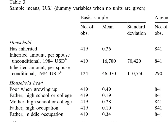
Table 3 presents averages for our two U.S. samples. The basic sample uses men and women who were household heads in 1984, who were at least 30 years old, who were not widows or widowers, whose parents were dead in 1984 (and, if married, all of whose spouse’s parents were dead as well), and who provided

9

amounts and years for all inheritances received. About 36% of the basic sample report receipt of an inheritance, the average per capita amount received is about $17,000, and the average amount conditional on receiving a positive inheritance is about $46,000.

Our ‘augmented sample’ combines past inheritances, including bracketed data,

9

(13)

Table 3

a

Sample means, U.S. (dummy variables when no units are given)

Basic sample Augmented sample

No. of Mean Standard No. of Mean Standard

obs. deviation obs. deviation

Household

Has inherited 419 0.36 841 0.42

Inherited amount, per spouse

b

unconditional, 1984 USD 419 16,780 70,420 841 22,860 65,160 Inherited amount, per spouse

b

conditional, 1984 USD 124 46,070 110,750 290 55,030 91,920 Household head

Poor when growing up 419 0.49 841 0.50

Father, high school or college 419 0.19 841 0.21 Mother, high school or college 419 0.28 841 0.28

Father, high occupation 419 0.10 841 0.10

Father, middle occupation 419 0.34 841 0.34

Lifetime earnings, 419 869,030 436,940 841 847,480 418,820

c

net of taxes, 1984 USD

Number of siblings 419 4.16 4.16 841 4.05 3.25

Age, years 419 59.1 10.1 841 61.0 10.5

Woman 419 0.31 841 0.26

Married 419 0.59 841 0.65

Years of education 419 12.35 3.01 841 11.91 3.28

a

Weighted sample. Inheritance amounts are present values at respondent age 50.

b

Includes predictions from column 4, Table 7, for bracketed values — see text.

c

Includes hours adjustment on part-time earnings — see text.

10

with those anticipated for the next 10 years. As we add the anticipated amounts, we feel we can loosen our restrictions on parents being deceased without jeopardizing the completeness of inheritance records: in the augmented sample, either (i) the parents (including the parents of a spouse) were dead in 1984, (ii) the 1988 PSID reports all the parents are dead, or (iii) the respondent (and spouse) was (were both) older than 60 in 1984 (so that surviving parents were already very elderly in 1984). Modifying the selection criterion in this way almost doubles the sample. Making use of anticipations and bracketed amounts raises the percent of observations with inheritances over the basic sample from 36 to 42%, and it raises the unconditional inheritance amount by almost 50%. To derive Table 3

inheri-10

(14)

tance amounts for the incomplete data, we predict within available brackets using the equation of column 4, Table 7.

To understand the importance of using the bracketed and otherwise incomplete data in the U.S. case, note that, had we omitted it, the augmented sample would have had 87 fewer observations — all with positive inheritances. Thus, the number of observations in the ‘conditional inheritance’ row of Table 3 for the augmented sample would have been 203, and the weighted mean in the ‘has inherited’ row would have been 0.33. The average unconditional inheritance would have been $13,210, smaller than the $16,780 of the basic sample, rather than $22,860. The average conditional inheritance would have been $38,100, smaller than the $46,070 for the basic sample, and substantially less than the $55,030 reported in the table. Clearly, making special efforts to recover information on inheritances from incomplete records has a large payoff in terms of sample averages for the PSID.

We use annual earnings, for men and women separately, for 1967–1993 to estimate earnings dynamics equations exactly analogous to the Swedish case — using observations in the PSID with positive earnings. The earnings regression uses only observations from ages below 60 and above both 16 and years of education plus 6. We ran the regressions separately with weighted and unweighted data; Table 3 and all subsequent results labeled ‘weighted’ (‘unweighted’) use the former (latter) coefficients. For each individual with any earnings, using the estimated coefficients, we predict a random effect u , then his or her earnings ati

each age to 65 from the maximum of 16 and schooling years plus 6, and then the present value at age 50 of his or her lifetime earnings (in 1984 dollars). In the regressions and earnings predictions, we multiply any annual earning observation with h,1750 hours of work per year by 1750 /h, our intent being to capture the value of a respondent’s time endowment, as we did with the Swedish data. (For comparison purposes, we derived a separate set of regression results for actual earnings.) Before calculating lifetime present values, we remove Federal income taxes using statutory rate tables for each year, and we also make a general correction for state income taxes (see Laitner and Ohlsson, 1997, for details). Table 3 reports average net-of-tax lifetime earnings (in present value at age 50) of about $869,000 for the basic sample and $847,000 for the augmented sample.

3.3. Summary and comparisons

(15)

unconditional inheritances are 3.0% of after-tax lifetime earnings in Sweden, but 1.9% in the basic PSID sample, and 2.7% in the augmented sample). (iii) Among respondents who receive inheritances, the amount relative to lifetime earnings is higher in the U.S. (i.e., 4.5% in Sweden, 5.3% in the PSID basic sample, and 6.5% in the augmented sample).

4. Analysis

The main purpose of this paper is to empirically distinguish the most appropriate model of bequest behavior, and to see if Sweden and the U.S. are

*

perhaps different in this regard. We work with the latent variable T defined in Section 2, parents’ desired bequest in the absence of nonnegativity constraint (2). We use a Tobit framework. Among the four models of Section 2, our results ultimately provide some support for the altruistic or exchange models in terms of

c *

the estimated sign of ≠T /≠Y . Estimated parameter magnitudes, on the other hand, reject altruism condition (5).

For future reference, the form of our Tobit is

* * y , if y .0,

y5

H

(14)

0, otherwise,

where

*

y 5x?b 1 e, (15)

*

with y the observed inheritance, y the parents’ (latent) bequest in the absence of a nonnegativity constraint, x a vector including proxies for parent lifetime resources, child lifetime earnings, and demographic variables, ande the regression error term, capturing measurement error in y and inter-family differences in preferences (i.e., differences inlof Section 2). For instances in which we know a respondent inherited but do not know the amount, our likelihood function assumes

*

y [[0,`). For PSID cases with lower and upper brackets a and b (corrected by inheritance date for price level and discounting), respectively, on the inheritance

*

amount, we assume y [[a,b].

We analyze the Swedish and U.S. data separately.

4.1. Results for Sweden

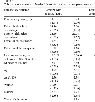
Table 4 shows Swedish outcomes for the Tobit of (14) and (15). Column 1 uses annual earnings with our adjustment to full-time work hours. The five independent variables starting with ‘poor when growing up’ capture the effect of parent lifetime resources. All four of our theoretical models imply ‘poor when growing up’ should

*

(16)

Table 4

a

Tobit: amount inherited, Sweden (absolute t-values within parentheses)

Explanatory variable Earnings with Earnings with adjusted hours actual hours

Poor when growing up 218.64 218.20 219.49 219.07

(2.87) (2.79) (3.55) (3.46)

Father, high school 14.44 12.04 12.01 8.92

or college (1.29) (1.05) (1.27) (0.92)

Mother, high school 24.19 22.78 26.05 23.62

or college (1.68) (1.57) (2.26) (2.02)

Father, high occupation 5.64 2.57 3.81 1.18

(0.35) (0.16) (0.28) (0.09)

Father, middle occupation 1.89 1.26 2.57 1.52

(0.29) (0.19) (0.46) (0.27)

Lifetime earnings, net 0.0168 0.0046 20.0057 20.0137

b

of taxes, 1000s 1984 USD (0.53) (0.13) (0.23) (0.55)

Number of siblings 22.71 22.60 22.91 22.75

Woman 11.50 10.33 5.81 4.96

(1.58) (1.40) (0.92) (0.78)

Married 217.83 217.72 212.55 212.52

(2.36) (2.34) (2.02) (2.02)

Years of education 1.13 1.31

(0.93) (1.33)

Constant 144.5 134.9 118.8 97.9

(1.29) (1.19) (1.29) (1.05)

1 / standard error 0.0158 0.0158 0.0171 0.0171

(25.8) (25.8) (28.2) (28.2)

No. of observations 509 616 616 616

2

x (11) 49.7493 50.6113 58.9770 60.7453

2

Pseudo-R 0.0122 0.0125 0.0123 0.0127

Log likelihood 22006.2 22365.8 22005.7 22365.0

a

Inherited amounts and life earnings present value age 50, 1000s 1984 USD.

b

Lifetime earnings present value age 50, 1000s, 1984 USD.

high socio-economic occupational status should have a positive effect. This is borne out: in the first column of Table 3, ‘poor when growing up’ implies a

*

$19,000 reduction in T , and having a mother with a high school education or *

more raises T by about $24,000. The other three parent variables have positive coefficients, though not statistically significant at the 10% level.

c

(17)

a $1 increase in a child’s earnings raises his inheritance by less than 2 cents. A coefficient insignificantly different from zero supports the egoistic and incomplete annuitization models.

c

There is reason, however, to fear that the coefficient of Y is upward biased. The logic is as follows. If our five proxy variables do not perfectly characterize parent

p p c

resources Y 1I , Y may well be positively correlated with the unexplained

c c

*

portion. Thus the coefficient of Y here may reflect not≠T /≠Y , but rather

* *

≠T ≠T

]]c 1a?]]p,

≠Y ≠Y

c p p

where a is the coefficient of Y in a regression of Y 1I on the independent variables of Table 3. An upward bias is likely because all inheritance theories

p *

imply ≠T /≠Y .0 and empirical work of Solon and others implies a.0. We return to this issue in Section 4.3.

Among the remaining variables, number of siblings and being married have a *

significantly negative effect on T .

Column 2 repeats the Tobit with child’s education included as a regressor. The coefficient on education is positive but not significant, and its inclusion has little effect on other coefficient estimates. Line 6 implies the coefficient should be negative. The importance of the Becker–Tomes analysis for Sweden is not clear at this point, and it remains a topic for future research.

c Columns 3 and 4 repeat the analysis using actual earnings in deriving Y rather than adjusting to full-time hours. Most coefficient estimates are quite similar to

c

columns 1 and 2. However, the coefficient on Y becomes negative, though still not significantly different from zero. The actual-hours figures may reflect legitimate differences in earning abilities, for instance because of disabilities, locational factors, or unwillingness to work long hours. Or they may lead to an endogeneity problem, with men and women who receive large inheritances tending to work shorter hours.

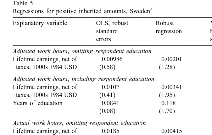
Table 5 presents regressions for Swedish respondents conditional on a positive inheritance. Column 1 provides OLS results (with White standard errors), column 2 results from a robust regression routine, and column 3 results from a median

11

regression (with bootstrapped standard errors). The regressors are the same as

c c

Table 5, although we omit most coefficients to concentrate on Y and E . The most interesting new finding is that, in all 12 of the conditional regressions, the coefficient of recipient’s lifetime earnings is negative. It is significantly different from 0 at the 5% level in about one-third of the cases. In all cases,

c

* however, its magnitude is small: raising Y by one dollar never decreases T by more than 2 cents.

11

(18)

Table 5

a

Regressions for positive inherited amounts, Sweden

Explanatory variable OLS, robust Robust Median regression, standard regression bootstrapped

errors standard errors

Adjusted work hours, omitting respondent education

Lifetime earnings, net of 20.00986 20.00201 20.00175 taxes, 1000s 1984 USD (0.58) (1.28) (0.73) Adjusted work hours, including respondent education

Lifetime earnings, net of 20.0107 20.00341 20.00464 taxes, 1000s 1984 USD (0.41) (1.95) (1.47)

Years of education 0.0841 0.118 0.171

(0.08) (1.70) (1.26)

Actual work hours, omitting respondent education

Lifetime earnings, net of 20.0185 20.00415 20.00451 taxes, 1000s 1984 USD (1.36) (2.88) (2.15) Actual work hours, including respondent education

Lifetime earnings, net of 20.0205 20.00506 20.00585 taxes, 1000s 1984 USD (1.50) (3.42) (2.58)

(0.51) (2.29) (1.18)

a

Inherited amounts and life earnings in 1000s USD. Absolute t-values within parentheses. Complete list of regressors as in Table 4.

4.2. Results for the U.S.

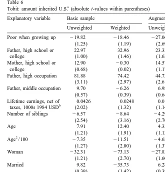
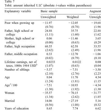
Tables 6 and 7 present results for our U.S. sample. Each table uses both our basic and augmented samples. Table 7 adds head’s education as a regressor. Recall that, for the PSID, weights can make a big difference, with weighted results mimicking a random sample much more closely.

Among the variables characterizing the parents, we have good agreement with our theories, all of which imply that high resource parents should leave larger estates. In the tables, ‘poor when growing up’ always has a negative sign, and it is statistically significant in the augmented sample. Being poor when young reduces one’s inheritance by $12–30,000. Father’s and mother’s education almost always has a positive effect as well, though only father’s education attains statistical significance at the 5% level, and only then in the weighted, augmented sample. Having a father with a high school education or more increases one’s inheritance by $23–36,000. Having a father with a very high occupational status yields a significantly positive effect in every column, the magnitude varying from $29 to 82,000.

(19)

Table 6

a

Tobit: amount inherited U.S. (absolute t-values within parentheses)

Explanatory variable Basic sample Augmented sample

Unweighted Weighted Unweighted Weighted Poor when growing up 219.82 218.46 227.06 229.55

(1.25) (1.19) (2.69) (3.12)

Father, high school or 22.97 32.96 23.33 26.49

college (1.00) (1.46) (1.63) (2.01)

Mother, high school or 12.90 20.30 14.57 8.88

college (0.68) (0.02) (1.17) (0.80)

(3.11) (2.97) (2.61) (2.53)

(0.57) (0.39) (0.64) (0.83)

Lifetime earnings, net of 0.0426 0.0248 0.0156 0.0058

b

taxes, 1000s 1984 USD (2.02) (1.32) (1.14) (0.49)

(2.54) (3.16) (2.70) (3.08)

Age 7.91 12.40 4.33 4.90

(1.21) (1.91) (1.13) (1.34)

Married 9.82 235.73 6.28 217.56

(0.39) (1.42) (0.38) (1.11)

Constant 2292.6 2333.4 2135.2 297.3

(1.58) (1.82) (1.25) (0.95)

1 / standard error 0.0087 0.0085 0.0093 0.0095

(14.8) (16.6) (20.5) (23.2)

No. of obs. 419 419 841 841

2

x (11) 65.1622 63.5404 96.5014 96.0038

2

Pseudo-R 0.0360 0.0291 0.0287 0.0237

Log likelihood 2872.8 21060.4 21634.4 21978.1

a

b

Annual earnings adjusted to full-time hours — see text.

statistical significance. The estimate draws even closer to 0 in the augmented sample.

As with the Swedish data, siblings affect one’s inheritance negatively. Being married does not have a significant negative effect in the U.S. case, but being female does. The latter is surprising and may be related to the fact that all of the female respondents in the U.S. data are single, and that since we attribute half of each couple’s total inheritance to the family head, married heads have higher odds of receiving a positive transfer.

(20)

Table 7

a

Tobit: amount inherited U.S. (absolute t-values within parentheses)

Explanatory variable Basic sample Augmented sample

Unweighted Weighted Unweighted Weighted Poor when growing up 211.97 212.05 219.68 222.88

(0.76) (0.78) (1.96) (2.41)

college (1.11) (1.60) (1.62) (2.04)

college (0.00) (0.63) (0.29) (0.00)

(2.62) (2.49) (1.96) (1.88)

(0.02) (0.79) (0.10) (1.40)

b

taxes, 1000s 1984 USD (1.07) (0.63) (0.04) (0.24)

(2.10) (2.76) (2.23) (2.55)

Age 8.04 11.70 4.34 4.59

(1.24) (1.81) (1.15) (1.28)

Married 14.06 227.19 5.16 213.72

(0.56) (1.08) (0.32) (0.88)

Years of education 8.65 7.74 6.62 6.11

(2.97) (2.74) (3.95) (3.73)

Constant 2385.5 2405.2 2208.5 2166.7

(2.07) (2.21) (1.93) (1.62)

1 / standard error 0.0088 0.0086 0.0094 0.0096

(14.9) (16.6) (20.6) (23.3)

No. of obs. 419 419 841 841

2

x (12) 74.2712 71.1570 112.4260 110.0820

2

Pseudo-R 0.0410 0.0326 0.0334 0.0272

Log likelihood 2868.2 21056.6 21626.4 21971.0

a

b

Annual earnings adjusted to full-time hours — see text.

difference than in the Swedish case. In contrast to the prediction of (6), our estimates of its coefficient are always positive. They are highly significant. According to the findings, another year of education adds $6–9000 to a child’s inheritance. As we move to the bigger sample and include weights, the magnitude of the coefficient declines slightly.

Including child’s education reduces the estimated coefficient on child’s earnings in every column. In fact, in the last column of Table 7 the estimated coefficient of

c c

(21)

positively related to the unexplained component of parent resources, and its inclusion in the regression may lower the bias on our estimated coefficient for child’s lifetime earnings.

Using actual rather than adjusted earnings makes virtually no difference in the U.S. case. Hence, we omit separate Tobit results for actual child earnings. Using weights evidently does make some difference, and this may be a signal that not all households have the same preferences, and that our econometric specification is not able to accommodate the heterogeneity.

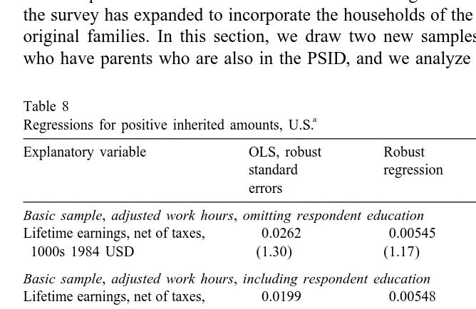
Table 8 studies the U.S. subsample with positive inheritances using robust and c

median regressions. The magnitude of the coefficient on Y tends to shrink and to lose its statistical significance. (Note that two of our three robust routines take only unweighted data, so that all comparisons to Tables 6 and 7 refer to columns 1 and 3 of the latter.) In contrast to the Swedish data, only one sign change emerges.

4.3. Further results for the U.S.

A unique feature of the PSID is that over its long duration, whenever possible the survey has expanded to incorporate the households of the grown children of its original families. In this section, we draw two new samples of household heads who have parents who are also in the PSID, and we analyze them jointly with the

Table 8

a

Regressions for positive inherited amounts, U.S.

Explanatory variable OLS, robust Robust Median regression, standard regression bootstrapped

errors standard errors

Basic sample, adjusted work hours, omitting respondent education

Lifetime earnings, net of taxes, 0.0262 0.00545 0.00574

1000s 1984 USD (1.30) (1.17) (0.71)

Basic sample, adjusted work hours, including respondent education

1000s 1984 USD (1.06) (1.20) (0.79)

(2.17) (0.88) (1.28)

Augmented sample, adjusted work hours, omitting respondent education

1000s 1984 USD (0.34) (1.82) (0.74)

Augmented sample, adjusted work hours, including respondent education

1000s 1984 USD (0.09) (1.28) (0.18)

(2.49) (1.33) (1.39)

a

(22)

samples of Table 3. We already have a good measurement of lifetime resources for households which inherit, and the new analysis helps us to pin down better the resources of the same households’ parents. There are three potential benefits: (i) we can assess our proxies for parent lifetime resources; (ii) our proxies are surely imperfect and a two-sample approach can reduce the bias on our estimate of the

c

crucial coefficient of Y above; and (iii) the new approach allows us explicitly to test condition (5). No analogue of the new steps, unfortunately, is possible with the Swedish LLS.

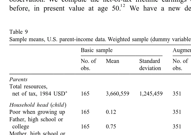
Table 9 presents averages for our additional U.S. samples. Each uses heads from 1984 (or spouses from 1984 who became heads in 1988 or 1993), who were children in 1968 of participating households, whose parents remained alive and in the PSID in 1984, and both of whose parents had at least one PSID earnings observation. We compute the net-of-tax lifetime earnings of the 1984 head as

12

before, in present value at age 50. We have a new dependent variable for

Table 9

Sample means, U.S. parent-income data. Weighted sample (dummy variables when no units are given) Basic sample Augmented sample

No. of Mean Standard No. of Mean Standard

obs. deviation obs. deviation

Parents Total resources,

a

net of tax, 1984 USD 165 3,660,559 1,245,459 351 3,148,365 1,596,895 Household head (child )

Poor when growing up 165 0.12 351 0.15

Father, high school or

college 165 0.75 351 0.69

Mother, high school or

college 165 0.81 351 0.78

Father, high occupation 165 0.33 351 0.25

Father, middle occupation 165 0.33 351 0.40 Lifetime earnings, net

b

of taxes, 1984 USD 165 1,180,043 496,434 351 1,155,923 539,32

Number of siblings 165 3.27 2.60 351 3.07 2.40

Age, years 165 30.2 4.99 351 30.9 4.77

Woman 165 0.35 351 0.33

Married 165 0.49 351 0.48

Years of education 165 13.9 2.22 351 14.0 2.28

a

Father’s and mother’s net-of-tax lifetime earnings plus inheritances, present value at date when child is 50. Includes hours adjustment on part-time earnings — see text.

b

Present value when child is age 50. Includes hours adjustment on part-time earnings.

12

(23)

analysis: we compute the net-of-tax lifetime earnings of both parents, sum the amounts, and add the parent household’s 1984 inheritance figure. The sum of the three figures constitutes the parent household’s ‘total resources.’ We want parents’ finished lifetime inheritances insofar as possible. Thus, our ‘basic parent-income sample’ includes only heads whose grandparents were all deceased by 1984 and whose household inheritance data is complete. Our ‘augmented parent-income sample’ adds to parents’ past inheritances the amounts which parents in 1984 anticipate inheriting over the next 10 years, uses records with bracketed and otherwise incomplete inheritance data, and includes heads (i) whose grandparents were all deceased by 1988 or (ii) whose parents were both older than 60 in 1984. As in Table 3, the augmented sample is considerably larger than the basic one. For Table 9, we impute parent total resources in cases of incomplete (parent) inheritance data (for the augmented sample) by estimating Eq. (17) below with a censored-normal regression and then computing the expected value of parent total resources conditional on available information. Finally, we compute the present value of the total resources of each head’s parents at the date the head is age 50

13 (recall the discussion of condition (5) in Section 2).

The equation we would like to estimate is

* * 9

y1i5y2i?p 1zi?g 1 ji, (16)

*

where y1i is the latent inheritance of child i (recall that negative desired *

inheritances are unobservable because of constraint (2)), y2i is the lifetime resources of the child’s parents, and z is a vector including the child’s lifetimei

earnings, a constant, and demographic information for the child (i.e., number of siblings, age, age squared, woman, married, and, perhaps, years of education). As

*

the samples of Table 3 do not include y , we now consider in addition a second2i equation to be estimated from the data of Table 9:

*

y2j5xj?a 1hj, (17)

*

where y2j is ‘total lifetime resources’ of the parent household of child j (i.e., the sum of the father’s lifetime earnings, the mother’s lifetime earnings, and the parent household’s lifetime inheritance), and where x is a vector including our five proxyj

variables of parent resources (i.e., was the child poor when growing up, did the child’s father have a high school education or more, did the child’s mother have a high school education or more, did the child’s father have a high-status occupation, and did the child’s father have a middle-status occupation), the child’s

13

(24)

c

lifetime earnings, x below, a constant, and our demographic information for childj

j. In cases with complete information about the parent’s inheritance, we observe *

y2j in our new sample(s). If the inheritance information is incomplete, we observe, *

say, a,b with y2j[[a,b). *

Returning to (16), although y2i is not observable in the data of Table 3, the elements of x (see the description of x above) are. Substituting from (17) intoi j

(16):

* 9

y1i5[xi?a 1hi]?p 1zi?g 1 ji. (18)

An assumption thathiis independent of each element of x insures the same is truei

with respect to z , which is a subvector of x . Lettingi i imposing the (cross-equation) restriction thata be the same in both equations. We estimate the joint likelihood function using our basic or augmented sample from Table 9 for (17) and from Table 3 for (19). Note that we need a censored-normal statistical model for (17) because not all of the parent-inheritance data is complete, and that we need a censored-normal Tobit for (19) because not all of the child-inheritance data is complete and because in (19) we want to model latent

14 inheritances, for which negative values are unobservable.

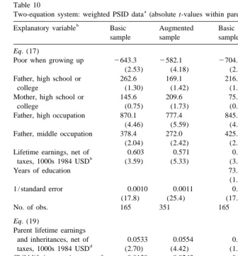
Table 10 presents the results. As weighted data seem the most interesting in the case of the PSID, we present weighted regressions with and without child education. Although each x , x , and z includes a constant, head’s number ofi j j

siblings, head’s age, age squared, head female, and head married in 1984, Table 10 omits coefficient estimates for the latter variables to save space.

The top of Table 10 shows that estimated coefficients for our proxy variables do produce the expected sign pattern in predicting parent lifetime resources. In column 2, for instance, being poor when growing up lowers the predicted total resources of one’s parents by about 580,000 USD, having an educated father raises the total resources of one’s parents by 170,000 USD, having an educated mother raises them 210,000 USD, and having a father with a high-status occupation raises them about 780,000 USD. Many of the estimated coefficients are statistically significant, especially in the case of the larger, augmented sample. (Note that we

14

*

Notice that we want the parent household’s actual inheritance as a component of y2j in (17),

*

(25)

Table 10

a

Two-equation system: weighted PSID data (absolute t-values within parentheses)

b

Explanatory variable Basic Augmented Basic Augmented

sample sample sample sample

Eq. (17)

Poor when growing up 2643.3 2582.1 2704.3 2590.4

(2.53) (4.18) (2.58) (3.96)

college (1.30) (1.42) (1.00) (1.14)

college (0.75) (1.73) (0.36) (1.05)

(4.46) (5.59) (4.24) (5.33)

(2.04) (2.42) (2.20) (2.31)

b

taxes, 1000s 1984 USD (3.59) (5.33) (3.04) (4.51)

(1.77) (1.97)

1 / standard error 0.0010 0.0011 0.0011 0.0011

(17.8) (25.4) (17.9) (25.5)

No. of obs. 165 351 165 351

Eq. (19)

Parent lifetime earnings

and inheritances, net of 0.0533 0.0554 0.0371 0.0432

d

taxes, 1000s 1984 USD (2.70) (4.42) (1.95) (3.30) Child lifetime earnings, net of 20.0139 20.0263 20.0145 20.0249

taxes, 1000s 1984 USD (0.57) (1.67) (0.66) (1.70)

(1.37) (1.49)

1 / standard error 0.0083 0.0094 0.0084 0.0095

(16.4) (23.2) (16.6) (23.2)

No. of obs. 419 841 419 841

2 c

x (18 or 20) 143.0630 213.8750 137.2880 230.3070

2

Pseudo-R 0.0286 0.0225 0.0274 0.0242

Log likelihood 22430.8 24653.6 22433.7 24645.4

a

Inheritances and lifetime earnings in 1000s 1984 USD.

b 2

Each equation also included a constant, number of siblings, age, age / 100, woman, and married as regressors. The table omits these for the sake of brevity.

c

Likelihood ratio statistic testing complete model versus a constant alone for each equation.

d

I.e., xj?a from (17).

either use our basic samples for both (17) and (19) or our augmented samples for both equations.)

Despite the sensible results for the five proxy variables which we depended on

p p c

(26)

parent earnings, even after including the five proxies for parents, suggests the c

coefficients for Y in Table 6 may be seriously biased.

Shifting attention to the bottom of Table 10, the coefficient estimates for parent lifetime resources, p in (19), are positive in every column, and statistically

p *

significant at the 5% level. Since p 5 ≠T /≠Y , this means our estimate of the latter is positive, which is consistent with all of our theoretical models of intergenerational transfers.

The coefficient estimate for ‘child lifetime earnings’ at the bottom of Table 10 c

refers to the first element ofg in (19) (i.e., the coefficient of x in z ). We havei i

c *

g 5 ≠1 T /≠Y . We can see the magnitude of the problem with our estimates in Section 4.2: the regressions based on (15) in Section 4.2 effectively estimate (19)

c

by itself, without (17); hence, the coefficient of Y in (15) corresponds to

a ? p 1 g6 1 (20)

c

in (17), witha6the coefficient of x in x . Our estimate ofi i a6is always positive at the top of Table 10, andp .0 at the bottom; hence, estimates of (20) provide a severely upwardly biased estimate ofg1.

This section eliminates the problem by estimating (17) and (19) together, thereby separately identifyingg1. Having done this, we find that our estimates of

c *

g 5 ≠1 T /≠Y at the bottom of Table 10 are uniformly negative. The estimates are statistically significantly different from zero at the 10% level for the augmented samples in columns 2 and 4. According to the estimates, parents drop their latent transfer by 1.5–2.5 cents for every dollar increase in their child’s lifetime earnings. The last two columns of Table 10 show that the magnitude of the estimated coefficient of child’s education in the inheritance equation falls by 50% or more from Table 7, and it ceases to be statistically significantly different from zero.

We conclude that, in terms of coefficient signs, the bottom half of Table 10 supports the altruistic model of intergenerational transfers — or the exchange model. Our discussion leads us to expect, under altruism, a negative coefficient on child’s education as well, and that is not supported, although our most sophisti-cated treatment reveals an estimated coefficient insignificantly different from zero. As noted, the education variable may be correlated with parental altruism. This remains a topic for further research.

p c

* *

(27)

Table 11

Point estimates and confidence intervals for condition (5)

Sample Point estimate Confidence interval

* *

≠T ≠T

]p2]c 95% 99%

≠Y ≠Y

Basic sample, 0.0672 (20.0138, 0.1482) (20.0437, 0.1781) omitting head’s education

Augmented sample, 0.0817 (0.0290, 0.1345) (0.0095, 0.1540) omitting head’s education

Basic sample, 0.0516 (20.0202, 0.1234) (20.0464, 0.1496) including head’s education

Augmented sample, 0.0681 (0.0182, 0.1179) (0.0001, 0.1360) including head’s education

5. Conclusion

We have analyzed two data sets, one for Sweden and one for the U.S. We find that inheritances are smaller but more widespread in Sweden. That, however, may be due to differences in the tax treatment of bequests in the two countries. A comparison of behavior in the two — see, for example, Tables 4, 6 and 7 — suggests that preference orderings may be fairly similar.

Our results on bequest behavior offer some support for the altruistic model: as we work to develop larger samples and to reduce biases in our estimates, the sign pattern the model predicts — inheritances positively related to donors’ lifetime resources but negatively related to heirs’ earning potentials — emerges, with marginally significant coefficients. This model is, of course, very widely used in macroeconomic research. On the other hand, the magnitude of the effects which we estimate is much smaller than the altruistic theory implies. In light of other recent work by Altonji et al., it seems likely that our result on magnitudes would stand even if we combined inter vivos and post-mortem transfers. Our experiments with education transfers do not seem encouraging for the theory at this point either. Possibly the exchange model ultimately fits the data better than altruism. Alternatively, perhaps a mixture of behaviors is present in the data, with some families following the altruistic model but others the egoistic or accidental models. (Differences between results with weighted and unweighted data in Tables 6 and 7 may also suggest heterogeneity.)

(28)

points to a possible endogeneity problem for children’s education and, in the Swedish case, for work hours as well.

Acknowledgements

This paper was originally prepared for the International Seminar in Public Economics conference on Bequest and Wealth Taxation, 18–20 May 1998,

`

University of Liege, Belgium. Helpful comments from James Poterba and Anne `

Laferrere — our discussants — the conference participants, two anonymous referees, and the editor are gratefully acknowledged. The research was funded by the Bank of Sweden Tercentenary Foundation, grant 94-0094:01-03. Laitner thanks NIA for partial support through grant AG 14898-01. Some of the work was

´ ´

done when Ohlsson enjoyed the hospitality of ERMES, Universite Pantheon-Assas, Paris II. We owe thanks to Ming Ching Luoh for help with the PSID data.

Appendix A. The data

Level of living survey

The LLS is collected by the Swedish Institute for Social Research, Stockholm University. The data are not directly publicly available. More information can be

˚

found in Erikson and Aberg (1987) or at http: / / www.sofi.su.se / sofipress.htm. Unless otherwise indicated, the data we have used are from the 1981 wave. Our variables are:

The respondent has inherited: variable U580 (1981 wave), V605 (1974 wave) and W377 (1968 wave).

Inherited amount at age 50 of the respondent. The nominal amounts and corresponding years are given by U581 and U582. We have also used the corresponding variables V606, V607 (1974 wave) and W378, W379 (1968 wave) to adjust the data.

Respondent’s parents deceased: U2151. Widowed respondent: U9053.

Respondent poor when growing up: U2551.

(29)

Number of siblings of the respondent: U28. Age of respondent: U11 gives the year of birth. Woman respondent: U1052.

Married, two spouses in the household: U9054.

Years of education. U137 reports the respondent’s years of education. We use the corresponding variables from the previous waves W538 (1968) and V229 (1974) to adjust the data.

Panel study of income dynamics

The PSID is collected by the Institute for Social Research, University of Michigan. It is an annual survey since 1968. The data can be found starting from http: / / www.isr.umich.edu / src / psid / index.html. Unless otherwise indicated, the data we have used are from the 1984 family file. Our variables are:

The household has inherited: variable V1093751.

Inherited amount at age 50 of the household head. The nominal amounts are given by the variables V10940 / V10945 and the corresponding years by V10939 / V10944. The amount is divided by 2 for households with two spouses. Parents deceased. These variables come from the 1988 family file. V15810 reports year of death of head’s father, V15824 head’s mother, V15867 wife’s father, and V15881 wife’s mother. We have adjusted for possible changes in head and wife of the household between 1984 and 1988. For households with a single head the variable ‘parents deceased’51 if the years of deaths for head parents are 1984 or before. For households with two spouses the variable ‘parents deceased’51 if the years of deaths for both spouses parents are 1984 or before.

Widowed head: V1042653.

Head poor when growing up: V1098851. Head’s father high occupation: V1097151 or 2. Head’s father middle occupation: V10971$3 and #5.

Head’s father secondary or college education. V10989$4 and #8. Head’s mother secondary or college education. V10990$4 and #8.

Lifetime earnings of the head, net of taxes. The earnings dynamics equations are estimated using data on annual labor income from the PSID 1968–1992 individual data set, the variables V30012 (1968)–V30750 (1992).

Number of siblings. These variables come from the 1986 family file. V13488 reports the head’s number of brothers and V13494 the head’s number of sisters. We have adjusted for possible changes in head and wife of the household between 1984 and 1986. V10979 in the 1984 survey reports the number of siblings of the head. If the variables above yield a missing value we have used this variable.

(30)

Woman head: V1042052.

Married, two spouses in the household: V1067051.

Head’s years of education. V10996 gives the head’s years of education except for postgraduate studies. If V1100351, we have added 3 years.

References

¨

Ahlroth, S., Bjorklund, A., Forslund, A., 1997. The output of the Swedish education sector. Review of Income and Wealth 43 (1), 89–104.

Altonji, J.G., Hayashi, F., Kotlikoff, L.J., 1992. Is the extended family altruistically linked? Direct tests using micro data. American Economic Review 82 (5), 1177–1198.

Altonji, J.G., Hayashi, F., Kotlikoff, L.J., 1997. Parental altruism and inter vivos transfers: theory and evidence. Journal of Political Economy 105 (6), 1121–1166.

`

Arrondel, L., Laferrere, A., 1998. Taxation and wealth transmission in France: some preliminary results. In: Paper presented at the ISPE conference on Bequest and Wealth Taxation, University of

` Liege, May.

Arrondel, L., Masson, A., Pestieau, P., 1997. Bequest and inheritance: empirical issues and France– U.S. comparison. In: Erreygers, G., Vandevelde, T. (Eds.), Is Inheritance Legitimate? Ethical and Economic Aspects of Wealth Transfers. Springer, Berlin, pp. 89–125, Chapter 4.

Barro, R.J., 1974. Are government bonds net wealth? Journal of Political Economy 82 (6), 1095–1117. Barthold, T.A., Ito, T., 1992. Bequest taxes and accumulation of household wealth: U.S.–Japan comparison. In: Ito, T., Krueger, A.O. (Eds.), The Political Economy of Tax Reform. NBER-East Asia Seminar on Economics, Vol. 1. University of Chicago Press, Chicago, pp. 235–290. Becker, G.S., 1974. A theory of social interactions. Journal of Political Economy 82 (6), 1063–1093. Becker, G.S., Tomes, N., 1979. An equilibrium theory of the distribution of income and

intergenera-tional mobility. Journal of Political Economy 87 (6), 1153–1189.

Bernheim, B.D., Bagwell, K., 1988. Is everything neutral? Journal of Political Economy 96 (2), 308–338.

Bernheim, B.D., Shleifer, A., Summers, L.H., 1985. The strategic bequest motive. Journal of Political Economy 93 (6), 1045–1076.

¨ ¨

Bjorklund, A., Jantti, M., 1997. Intergenerational income mobility in Sweden compared to the United States. American Economic Review 87 (5), 1009–1018.

Blanchflower, D.G., Oswald, A.J., 1998. What makes an entrepreneur? Journal of Labor Economics 16 (1), 26–60.

Blinder, A.B., 1974. Toward an Economic Theory of Income Distribution. MIT Press, Cambridge, MA. Chamley, C., 1986. Optimal taxation of capital income in general equilibrium with infinite lives.

Econometrica 54 (3), 607–622.

Cnossen, S., 1998. Wealth, inheritance and gift taxes in the OECD area. A survey. In: Paper presented `

at the ISPE conference on Bequest and Wealth Taxation, University of Liege, May.

Cox, D., 1987. Motives for private income transfers. Journal of Political Economy 95 (3), 508–546. Cox, D., Rank, M.R., 1992. Inter-vivos transfers and intergenerational exchange. Review of Economics

and Statistics 74 (2), 305–314.

Cremer, H., Pestieau, P., 1996. Bequests as heir ‘discipline device’. Journal of Population Economics 9 (4), 405–414.

Cremer, H., Pestieau, P., 1998. Non-linear taxation of bequests, equal sharing rules and the tradeoff between intra- and inter-family inequalities. In: Paper presented at the ISPE conference on Bequest

` and Wealth Taxation, University of Liege, April.